Atomistic simulation introduction
What is “atomistic simulation”, and what can be done with it? This section provides an overview.
Various properties of materials can be explained at the atomic level. For example, mechanical properties (elastic constants, Young’s modulus, etc.), thermophysical properties (specific heat, etc.), viscosity, chemical reactions, etc. Atomistic simulations can be used to reproduce how atoms move or to analyze how atoms are arranged in nature.
We will explain the detail gradually, but for now, let’s start with the following code.
Initial setup
The libraries required to run this tutorial can be installed by executing the following command in the Matlantis system.
pfp-api-clientmatlantis-featurespfcc-extras
are provided only inside Matlantis system.
※For pfcc-extras, please copy the package from “package launcher”, and install it by following the README.md located inside. ※After installing these libraries, you may need to restart the kernel to reflect the installation. If the subsequent import fails despite the installation succeeded log, try restarting the kernel by selecting “Restart kernel…” from the top tab.
[ ]:
!pip install -U pfp-api-client matlantis-features pfcc-extras
# !pip install -e ../pfcc-extras  # please specify the path
Executing simple MD simulation example
This is a sample MD (Molecular Dynamics) simulation for silicon dioxide (SiO2 crystal), a major component of the earth’s surface. At this point, you do not need to understand the code at all. Seeing is believing, so let’s run it and visualize it first. (By the end of this tutorial, you will be able to easily understand what this code is doing.)
[2]:
from ase.md.velocitydistribution import MaxwellBoltzmannDistribution, Stationary
from ase.md.verlet import VelocityVerlet
from ase.optimize import BFGS
from ase.io import Trajectory, read
from ase import units

from pfp_api_client.pfp.calculators.ase_calculator import ASECalculator
from pfp_api_client.pfp.estimator import Estimator, EstimatorCalcMode

estimator = Estimator(calc_mode=EstimatorCalcMode.PBE, model_version="v8.0.0")
calculator = ASECalculator(estimator)

atoms = read("../input/SiO2_mp-6930_conventional_standard.cif")
atoms.calc = calculator


opt = BFGS(atoms)
opt.run()

atoms = atoms * (3, 3, 3)
atoms.calc = calculator
# Set the momenta corresponding to T=700K.
MaxwellBoltzmannDistribution(atoms, temperature_K=700.0)
# Sets the center-of-mass momentum to zero.
Stationary(atoms)
# Run MD using the VelocityVerlet algorithm
dyn = VelocityVerlet(atoms, 1.0 * units.fs, trajectory="output/dyn.traj")

def print_dyn():
    print(f"Dyn  step: {dyn.get_number_of_steps(): >3}, energy: {atoms.get_total_energy():.3f}")

dyn.attach(print_dyn, interval=10)
dyn.run(100)
      Step     Time          Energy          fmax
BFGS:    0 07:05:37      -57.072312        0.010031
Dyn  step:   0, energy: -1519.718
Dyn  step:  10, energy: -1519.660
Dyn  step:  20, energy: -1519.668
Dyn  step:  30, energy: -1519.688
Dyn  step:  40, energy: -1519.674
Dyn  step:  50, energy: -1519.676
Dyn  step:  60, energy: -1519.682
Dyn  step:  70, energy: -1519.679
Dyn  step:  80, energy: -1519.678
Dyn  step:  90, energy: -1519.678
Dyn  step: 100, energy: -1519.681
[2]:
True
[3]:
from pfcc_extras.visualize.view import view_ngl

traj = Trajectory("output/dyn.traj")[::5]
view_ngl(traj, representations=["ball+stick"])
[3]:
[4]:
from pfcc_extras.visualize.povray import traj_to_gif, traj_to_apng
from IPython.display import Image


traj_to_apng(traj, "output/sio2-md.png", rotation="30x,30y,30z", clean=True, n_jobs=16, width=600)
Image(url="output/sio2-md.png")  # , width=150
[Parallel(n_jobs=16)]: Using backend ThreadingBackend with 16 concurrent workers.
[Parallel(n_jobs=16)]: Done  12 out of  21 | elapsed:   20.3s remaining:   15.2s
[Parallel(n_jobs=16)]: Done  21 out of  21 | elapsed:   26.0s finished
[4]:
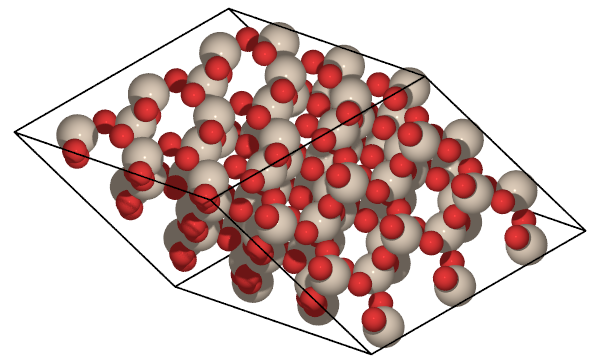
A technique called molecular dynamics is used to study the dynamics of atoms in SiO2 crystals at 700K.
In the above example, we simulated 243 atoms. The volume is about \(3 \times 10^{-27}\)m, and the length scale is about 15Å = (\(15 \times 10^{-10}\)m) for each axis, which is many orders of magnitude smaller than the 1m scale that we deal with in our daily lives.
One thing to consider here is that we cannot simulate on a computer the entire material we are dealing with on the same scale as it is. Even materials on the order of grams have Avogadro’s number, i.e., atoms on the order of \(10^{23}\), and the computer cannot handle such a large number of atoms.
Therefore, in atomistic simulations, it is necessary to perform appropriate modeling according to the phenomenon to create a simplified system that can be analyzed on a computer by extracting only the necessary elements to reproduce the desired phenomenon, rather than creating something exactly the same as the natural world. There are various methods for modeling, and you will be able to do them by learning through this tutorial.
[Column] Modeling
For example, if you want to simulate the Earth, if you are interested in weather, you would need to focus your modeling on the Earth’s surface atmosphere. On the other hand, if you are interested in earthquakes, you would need to concentrate your modeling on the Earth’s internal structure rather than the atmosphere. If you want to simulate the environment on the surface of the earth, you might consider cutting out only a portion of a continent rather than the entire planet.
Again, let’s look at the simulation results. The ones that appear here include the following.
Atom
Each atom is specified by element number, has an xyz coordinate value, and has a velocity.
Cell.
The box is represented by the cube in the above figure. It allows us to deal with systems in which this cell follows the periodic boundary condition indefinitely.
When dealing with a molecule floating in a vacuum, the cell periodic boundary condition is not necessary. For systems such as solids, which have a regular structure, the periodic boundary condition allows us to treat structures that extend infinitely in each of the x, y, and z axes (strictly speaking, the a, b, and c axes, which are the crystal axes).
The cell & periodic boundary condition are artificial concepts for the convenience of computation and modeling. In reality, a crystal structure is considered to have a regular structure in the interior followed by another structure on the surface. However the surface is in a very different state compared to interior and has special characteristics, making computation difficult in some cases. Therefore, by artificially limiting our simulation to the world of cells and imposing the periodic boundary condition that the right end and the left end are connected, we can create a world that has no surface and continues repeatedly, so that we can deal with problems.
In the next section, we will learn how to handle these structures with Python programs and perform atomistic simulations.