Reaction pathway analysis
In the previous chapters, we have been looking at the behavior near the stable structure. In this chapter, we will analyze the reaction of substances.

The relationship between the activation energy \(E_a\) and the enthalpy of reaction \(\Delta H\) associated with the reaction X→Y. Cited from Wikipedia.
In a reaction process in which product Y is formed from reactant X, the point with the maximum energy in the reaction path is called the Transition State (TS), and the energy difference between reactant/product and the transition state is called the Activation energy \(E_a\).
According to the Arrhenius equation, the reaction rate constant \(k\) is wrriten as
where
\(A\): pre-exponential factor (a constant independent of temperature)
\(E_a\): activation energy
\(k_B\): Boltzmann constant
\(T\): temperature
Thus, the likelihood of a chemical reaction is determined by the activation energy \(E_a\).
The energy of reactants/products does not change, but the activation energy changes as the reaction path changes with the surrounding environment, i.e., the presence of a catalyst. If we can find a catalyst with lower activation energy, we can make the target reaction more likely to be produced.
Reference:
Even if reactant X and product Y are known, finding the transition state is not obvious. In this section, we will try to calculate the activation energy using the NEB (Nudged Elastic Band) method, which searches for reaction pathways when the structures before and after the reaction are known.
NEB
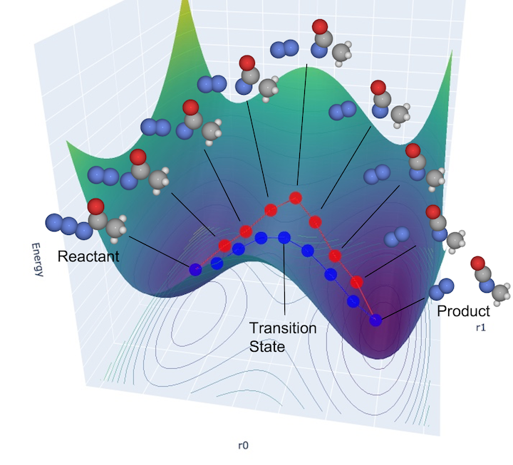
Diagram of the NEB method: After generating reaction path candidates (red line) as the initial configuration, structural relaxation is performed to search for reaction paths (blue line) that pass through transition states.
[Note] The following content is based on the NEB Tutorial in the Matlantis.
We will investigate an organic chemical reaction called the Curtius rearrangement.
In the NEB method, we usually start with preparing the structures before and after a particular chemical reaction of interest.
This time, we will write down the structures directly.
[1]:
import numpy as np
from IPython.display import Image
import matplotlib.pyplot as plt

import ase
from ase import Atoms
from ase.visualize import view
from ase.optimize import BFGS
from ase.optimize import FIRE
from ase.neb import NEB
from ase.build.rotate import minimize_rotation_and_translation

from pfp_api_client.pfp.calculators.ase_calculator import ASECalculator
from pfp_api_client.pfp.estimator import Estimator
from pfp_api_client.pfp.estimator import Estimator, EstimatorCalcMode

estimator = Estimator(calc_mode=EstimatorCalcMode.PBE, model_version="v8.0.0")
calculator = ASECalculator(estimator)
[2]:
react = ase.Atoms(
    symbols="C2NON2H3",
    positions = [
        [ 2.12, -0.48,  0.00],
        [ 0.76,  0.16, -0.00],
        [-0.28, -0.79, -0.00],
        [ 0.57,  1.35,  0.00],
        [-1.42, -0.28,  0.00],
        [-2.48,  0.07,  0.00],
        [ 2.67, -0.14, -0.88],
        [ 2.06, -1.57, -0.00],
        [ 2.67, -0.14,  0.88],
    ],
)

prod = ase.Atoms(
    symbols="C2NON2H3",
    positions=[
        [ 2.30, -0.87,  0.00],
        [ 0.68,  0.92, -0.00],
        [ 0.99, -0.25,  0.00],
        [ 0.25,  2.03,  0.00],
        [-2.34,  0.11,  0.00],
        [-3.13, -0.67, -0.00],
        [ 2.87, -0.57, -0.89],
        [ 2.19, -1.96,  0.00],
        [ 2.87, -0.57,  0.89],
    ],
)
The first step is to perform structural optimization. The way of structural optimization is the same as before.
To facilitate future work, we will move the structures before and after the reaction so that they are as close as possible. This is done by minimize_rotation_and_translation method.
[3]:
react.calc = calculator
opt = BFGS(react)
opt.run(fmax=0.01)

prod.calc = calculator
opt = BFGS(prod)
opt.run(fmax=0.01)

minimize_rotation_and_translation(react, prod)
      Step     Time          Energy          fmax
BFGS:    0 05:53:02      -41.413419        3.177696
BFGS:    1 05:53:07      -41.195533        8.812655
BFGS:    2 05:53:07      -41.470582        0.869362
BFGS:    3 05:53:07      -41.475647        0.802335
BFGS:    4 05:53:07      -41.480740        0.326584
BFGS:    5 05:53:07      -41.482541        0.187571
BFGS:    6 05:53:07      -41.484103        0.097033
BFGS:    7 05:53:08      -41.484652        0.066656
BFGS:    8 05:53:08      -41.485013        0.077300
BFGS:    9 05:53:08      -41.485479        0.091526
BFGS:   10 05:53:08      -41.485934        0.083387
BFGS:   11 05:53:08      -41.486403        0.071168
BFGS:   12 05:53:08      -41.486817        0.072329
BFGS:   13 05:53:08      -41.487162        0.050056
BFGS:   14 05:53:08      -41.487408        0.046723
BFGS:   15 05:53:08      -41.487569        0.033225
BFGS:   16 05:53:08      -41.487688        0.036092
BFGS:   17 05:53:08      -41.487823        0.039096
BFGS:   18 05:53:08      -41.487948        0.046989
BFGS:   19 05:53:08      -41.488031        0.031865
BFGS:   20 05:53:08      -41.488063        0.013554
BFGS:   21 05:53:09      -41.488073        0.012217
BFGS:   22 05:53:09      -41.488093        0.013953
BFGS:   23 05:53:09      -41.488106        0.019451
BFGS:   24 05:53:09      -41.488128        0.015627
BFGS:   25 05:53:09      -41.488135        0.006002
      Step     Time          Energy          fmax
BFGS:    0 05:53:09      -42.999059        0.928905
BFGS:    1 05:53:09      -42.979845        2.213718
BFGS:    2 05:53:09      -43.002931        0.183858
BFGS:    3 05:53:09      -43.002438        0.498714
BFGS:    4 05:53:09      -43.004179        0.132442
BFGS:    5 05:53:09      -43.005464        0.146250
BFGS:    6 05:53:09      -43.008521        0.384096
BFGS:    7 05:53:09      -43.011647        0.401999
BFGS:    8 05:53:10      -43.015385        0.276139
BFGS:    9 05:53:10      -43.018492        0.163363
BFGS:   10 05:53:10      -43.021307        0.250461
BFGS:   11 05:53:10      -43.023818        0.292535
BFGS:   12 05:53:10      -43.025384        0.156905
BFGS:   13 05:53:10      -43.026212        0.098028
BFGS:   14 05:53:10      -43.026830        0.146643
BFGS:   15 05:53:10      -43.027199        0.128298
BFGS:   16 05:53:10      -43.027410        0.062755
BFGS:   17 05:53:10      -43.027560        0.069153
BFGS:   18 05:53:10      -43.027842        0.149047
BFGS:   19 05:53:10      -43.028350        0.228853
BFGS:   20 05:53:10      -43.029111        0.244633
BFGS:   21 05:53:11      -43.030054        0.159354
BFGS:   22 05:53:11      -43.031161        0.120736
BFGS:   23 05:53:11      -43.032580        0.200826
BFGS:   24 05:53:11      -43.034554        0.315799
BFGS:   25 05:53:11      -43.036725        0.259742
BFGS:   26 05:53:11      -43.037638        0.081485
BFGS:   27 05:53:11      -43.037804        0.026730
BFGS:   28 05:53:11      -43.037886        0.024726
BFGS:   29 05:53:11      -43.037905        0.020094
BFGS:   30 05:53:11      -43.037905        0.007461
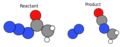
We check the reactant & product structures by visualization.
[4]:
from ase.io import write
from IPython.display import Image
import matplotlib.pyplot as plt
import matplotlib.image as mpimg

write("output/curtius_react.png", react, rotation="0x,0y,0z")
write("output/curtius_prod.png", prod, rotation="0x,0y,0z")

fig, axes = plt.subplots(1, 2, figsize=(6, 3))
ax0, ax1 = axes
ax0.imshow(mpimg.imread("output/curtius_react.png"))
ax0.set_axis_off()
ax0.set_title("Reactant")
ax1.imshow(mpimg.imread("output/curtius_prod.png"))
ax1.set_axis_off()
ax1.set_title("Product")
fig.show()
[5]:
from pfcc_extras.visualize.view import view_ngl

view_ngl([react, prod], representations=["ball+stick"], replace_structure=True)
[5]:
We will start to run NEB calculations from here. NEB is a method for finding reaction paths by interpolating many discrete structures between the structures before and after the reaction and then performing structural optimization on the combination of these structures in phase space.
We can use the functions in ASE for both interpolating the intermediate structure and performing NEB calculation. Note that in order to run the NEB calculation in parallel, we create a unique calculator instance for each structure, and specify allow_shared_calculator=False, parallel=True for NEB.
Because NEB contains multiple structures internally, the time cost of one step is greater than that of MD. Nevertheless, such a calculation can be completed in a few minutes with PFP, compared to several days or months with quantum chemical computation, e.g. DFT.
The calculations are performed in the following steps
First, create a list of ASE atoms as
images.The first one is the reactant
react, and the last one is the productprod.The coordinates of intermediate
imagewill be changed later with theneb.interpolate()method. Here, we only need to make a copy here.In this case, we have created 7 intermediate images, for a total of 9 images.
Create and set a
calculatorfor each atoms.Create NEB class
kis the spring constant that represents the strength of the spring connecting eachimages.By setting
climb=True, we use the Climbing Image NEB method, which is a method that reverts the energy gradient to find transition states.
neb.interpolate()Linear interpolation of the
imagesis executed to create a list of coordinates that gradually change from reactant to product.The initial configuration (candidates) of the reaction paths can be confirmed by commenting out the line with
view_ngl.
optimization with
FIREThe obtained reaction pathway candidates are modified to the appropriate reaction pathway by optimizing them using the
FIREmethod.
[6]:
images = [react.copy()]
images += [react.copy() for i in range (7)]
images += [prod.copy()]
for image in images:
    estimator = Estimator(calc_mode=EstimatorCalcMode.PBE, model_version="v8.0.0")
    calculator = ASECalculator(estimator)
    image.calc = calculator
neb = NEB(images, k=0.1, climb=True, allow_shared_calculator=False, parallel=True)
neb.interpolate()
# Check interpolated images
# view_ngl(images, representations=["ball+stick"], replace_structure=True)
opt = FIRE(neb)
status = opt.run(fmax=0.05, steps=500)
      Step     Time          Energy          fmax
FIRE:    0 05:53:17      -36.039934       51.039993
/tmp/ipykernel_38727/1903780971.py:8: FutureWarning: Please import NEB from ase.mep, not ase.neb.
  neb = NEB(images, k=0.1, climb=True, allow_shared_calculator=False, parallel=True)
FIRE:    1 05:53:17      -38.793782        9.718599
FIRE:    2 05:53:18      -38.639883       11.420030
FIRE:    3 05:53:18      -39.024515        7.290823
FIRE:    4 05:53:18      -39.146942        7.625532
FIRE:    5 05:53:18      -39.187412        5.992777
FIRE:    6 05:53:18      -39.239850        3.735237
FIRE:    7 05:53:18      -39.275642        3.622289
FIRE:    8 05:53:18      -39.291292        3.493045
FIRE:    9 05:53:18      -39.304292        4.473294
FIRE:   10 05:53:19      -39.331143        4.526304
FIRE:   11 05:53:19      -39.372896        3.701372
FIRE:   12 05:53:19      -39.419352        2.238812
FIRE:   13 05:53:19      -39.443115        2.080150
FIRE:   14 05:53:19      -39.440229        3.654853
FIRE:   15 05:53:19      -39.444635        2.844699
FIRE:   16 05:53:19      -39.441267        1.513861
FIRE:   17 05:53:19      -39.386240        2.479679
FIRE:   18 05:53:20      -39.331586        1.880054
FIRE:   19 05:53:20      -39.281403        1.779987
FIRE:   20 05:53:20      -39.283645        1.548858
FIRE:   21 05:53:20      -39.287574        1.518645
FIRE:   22 05:53:20      -39.292569        1.468452
FIRE:   23 05:53:20      -39.298437        1.397878
FIRE:   24 05:53:20      -39.305505        1.310686
FIRE:   25 05:53:20      -39.314064        1.211725
FIRE:   26 05:53:21      -39.323960        1.103863
FIRE:   27 05:53:21      -39.335856        0.975578
FIRE:   28 05:53:21      -39.349554        0.838575
FIRE:   29 05:53:21      -39.365411        0.882636
FIRE:   30 05:53:21      -39.383477        0.645287
FIRE:   31 05:53:21      -39.402059        0.823016
FIRE:   32 05:53:21      -39.419176        0.710753
FIRE:   33 05:53:21      -39.432073        0.612654
FIRE:   34 05:53:22      -39.435664        0.673938
FIRE:   35 05:53:22      -39.429984        0.665475
FIRE:   36 05:53:22      -39.417316        0.741882
FIRE:   37 05:53:22      -39.409039        0.755364
FIRE:   38 05:53:22      -39.416518        0.662316
FIRE:   39 05:53:22      -39.450880        0.688317
FIRE:   40 05:53:22      -39.504750        1.002623
FIRE:   41 05:53:22      -39.531253        1.980011
FIRE:   42 05:53:22      -39.531704        1.053129
FIRE:   43 05:53:23      -39.515310        1.783475
FIRE:   44 05:53:23      -39.516177        1.343500
FIRE:   45 05:53:23      -39.516109        0.887946
FIRE:   46 05:53:23      -39.513257        0.844553
FIRE:   47 05:53:23      -39.507936        0.981732
FIRE:   48 05:53:23      -39.502429        1.231033
FIRE:   49 05:53:23      -39.498270        1.107979
FIRE:   50 05:53:23      -39.495246        0.670416
FIRE:   51 05:53:24      -39.491761        0.478543
FIRE:   52 05:53:24      -39.487278        0.836828
FIRE:   53 05:53:24      -39.484502        0.931134
FIRE:   54 05:53:24      -39.485000        0.400947
FIRE:   55 05:53:24      -39.486132        0.687748
FIRE:   56 05:53:24      -39.488696        0.821196
FIRE:   57 05:53:24      -39.494420        0.299127
FIRE:   58 05:53:24      -39.498288        0.816078
FIRE:   59 05:53:25      -39.498931        0.651060
FIRE:   60 05:53:25      -39.499640        0.370306
FIRE:   61 05:53:25      -39.499844        0.387021
FIRE:   62 05:53:25      -39.499683        0.589927
FIRE:   63 05:53:25      -39.499753        0.568230
FIRE:   64 05:53:25      -39.499868        0.526476
FIRE:   65 05:53:25      -39.500018        0.468053
FIRE:   66 05:53:25      -39.500167        0.398406
FIRE:   67 05:53:26      -39.500278        0.325589
FIRE:   68 05:53:26      -39.500354        0.260600
FIRE:   69 05:53:26      -39.500395        0.295316
FIRE:   70 05:53:26      -39.500428        0.356153
FIRE:   71 05:53:26      -39.500498        0.391886
FIRE:   72 05:53:26      -39.500609        0.391706
FIRE:   73 05:53:26      -39.500797        0.348149
FIRE:   74 05:53:26      -39.501020        0.262223
FIRE:   75 05:53:26      -39.501209        0.304671
FIRE:   76 05:53:27      -39.501368        0.373761
FIRE:   77 05:53:27      -39.501593        0.386780
FIRE:   78 05:53:27      -39.501939        0.319477
FIRE:   79 05:53:27      -39.502316        0.236664
FIRE:   80 05:53:27      -39.502740        0.306992
FIRE:   81 05:53:27      -39.503442        0.221052
FIRE:   82 05:53:27      -39.504365        0.286691
FIRE:   83 05:53:28      -39.505714        0.257210
FIRE:   84 05:53:28      -39.507617        0.223562
FIRE:   85 05:53:28      -39.510176        0.142952
FIRE:   86 05:53:28      -39.513237        0.251855
FIRE:   87 05:53:28      -39.516656        0.249104
FIRE:   88 05:53:28      -39.519980        0.291716
FIRE:   89 05:53:28      -39.522918        0.423171
FIRE:   90 05:53:28      -39.525657        0.933060
FIRE:   91 05:53:28      -39.525950        0.122988
FIRE:   92 05:53:29      -39.526037        0.827977
FIRE:   93 05:53:29      -39.526125        0.630574
FIRE:   94 05:53:29      -39.526228        0.290080
FIRE:   95 05:53:29      -39.526321        0.146086
FIRE:   96 05:53:29      -39.526328        0.139804
FIRE:   97 05:53:29      -39.526347        0.127774
FIRE:   98 05:53:29      -39.526365        0.111241
FIRE:   99 05:53:29      -39.526388        0.109090
FIRE:  100 05:53:30      -39.526415        0.108170
FIRE:  101 05:53:30      -39.526451        0.107064
FIRE:  102 05:53:35      -39.526499        0.105773
FIRE:  103 05:53:35      -39.526544        0.112183
FIRE:  104 05:53:35      -39.526615        0.116831
FIRE:  105 05:53:35      -39.526700        0.118117
FIRE:  106 05:53:35      -39.526804        0.114901
FIRE:  107 05:53:35      -39.526934        0.107102
FIRE:  108 05:53:36      -39.527096        0.096492
FIRE:  109 05:53:36      -39.527287        0.098161
FIRE:  110 05:53:36      -39.527524        0.105876
FIRE:  111 05:53:36      -39.527818        0.109156
FIRE:  112 05:53:36      -39.528161        0.108226
FIRE:  113 05:53:36      -39.528585        0.107816
FIRE:  114 05:53:36      -39.529099        0.114348
FIRE:  115 05:53:36      -39.529700        0.128953
FIRE:  116 05:53:37      -39.530423        0.141629
FIRE:  117 05:53:37      -39.531288        0.141220
FIRE:  118 05:53:37      -39.532314        0.137819
FIRE:  119 05:53:37      -39.533546        0.148716
FIRE:  120 05:53:37      -39.535015        0.148140
FIRE:  121 05:53:37      -39.536748        0.124585
FIRE:  122 05:53:37      -39.538754        0.141570
FIRE:  123 05:53:37      -39.540931        0.334313
FIRE:  124 05:53:38      -39.542964        0.872740
FIRE:  125 05:53:38      -39.543108        0.099246
FIRE:  126 05:53:38      -39.543123        0.801354
FIRE:  127 05:53:38      -39.543166        0.608250
FIRE:  128 05:53:38      -39.543222        0.276952
FIRE:  129 05:53:38      -39.543266        0.167962
FIRE:  130 05:53:38      -39.543263        0.159837
FIRE:  131 05:53:38      -39.543266        0.144121
FIRE:  132 05:53:39      -39.543273        0.121977
FIRE:  133 05:53:39      -39.543288        0.108850
FIRE:  134 05:53:39      -39.543294        0.097559
FIRE:  135 05:53:39      -39.543311        0.086447
FIRE:  136 05:53:39      -39.543328        0.090467
FIRE:  137 05:53:39      -39.543352        0.099416
FIRE:  138 05:53:39      -39.543379        0.105308
FIRE:  139 05:53:40      -39.543413        0.106516
FIRE:  140 05:53:40      -39.543449        0.101807
FIRE:  141 05:53:40      -39.543505        0.091059
FIRE:  142 05:53:40      -39.543559        0.084905
FIRE:  143 05:53:40      -39.543637        0.096808
FIRE:  144 05:53:40      -39.543725        0.101426
FIRE:  145 05:53:40      -39.543840        0.093861
FIRE:  146 05:53:40      -39.543970        0.076909
FIRE:  147 05:53:41      -39.544133        0.090605
FIRE:  148 05:53:41      -39.544324        0.085783
FIRE:  149 05:53:41      -39.544556        0.078244
FIRE:  150 05:53:41      -39.544833        0.084897
FIRE:  151 05:53:41      -39.545156        0.070795
FIRE:  152 05:53:41      -39.545549        0.080475
FIRE:  153 05:53:41      -39.546006        0.079829
FIRE:  154 05:53:41      -39.546542        0.066319
FIRE:  155 05:53:42      -39.547176        0.067482
FIRE:  156 05:53:42      -39.547931        0.083006
FIRE:  157 05:53:42      -39.548789        0.205813
FIRE:  158 05:53:42      -39.549665        0.591954
FIRE:  159 05:53:42      -39.549807        0.069105
FIRE:  160 05:53:42      -39.549764        0.546293
FIRE:  161 05:53:42      -39.549809        0.415580
FIRE:  162 05:53:42      -39.549869        0.190804
FIRE:  163 05:53:42      -39.549892        0.139658
FIRE:  164 05:53:43      -39.549892        0.133200
FIRE:  165 05:53:43      -39.549899        0.120721
FIRE:  166 05:53:43      -39.549903        0.103139
FIRE:  167 05:53:43      -39.549910        0.081804
FIRE:  168 05:53:43      -39.549919        0.073125
FIRE:  169 05:53:43      -39.549927        0.066290
FIRE:  170 05:53:43      -39.549937        0.068883
FIRE:  171 05:53:43      -39.549953        0.079353
FIRE:  172 05:53:43      -39.549967        0.090279
FIRE:  173 05:53:44      -39.549984        0.092056
FIRE:  174 05:53:44      -39.550013        0.082493
FIRE:  175 05:53:44      -39.550042        0.069312
FIRE:  176 05:53:49      -39.550080        0.068212
FIRE:  177 05:53:49      -39.550123        0.076010
FIRE:  178 05:53:49      -39.550180        0.079268
FIRE:  179 05:53:49      -39.550251        0.075107
FIRE:  180 05:53:50      -39.550338        0.064926
FIRE:  181 05:53:50      -39.550441        0.074295
FIRE:  182 05:53:50      -39.550568        0.070558
FIRE:  183 05:53:50      -39.550722        0.070874
FIRE:  184 05:53:50      -39.550914        0.076569
FIRE:  185 05:53:50      -39.551142        0.064690
FIRE:  186 05:53:50      -39.551415        0.071405
FIRE:  187 05:53:50      -39.551746        0.075358
FIRE:  188 05:53:51      -39.552141        0.063727
FIRE:  189 05:53:51      -39.552616        0.065579
FIRE:  190 05:53:51      -39.553177        0.080591
FIRE:  191 05:53:51      -39.553823        0.147884
FIRE:  192 05:53:51      -39.554451        0.450631
FIRE:  193 05:53:51      -39.553907        1.523635
FIRE:  194 05:53:51      -39.555313        0.447544
FIRE:  195 05:53:51      -39.555376        0.315242
FIRE:  196 05:53:51      -39.555435        0.099751
FIRE:  197 05:53:52      -39.555439        0.194017
FIRE:  198 05:53:52      -39.555440        0.181617
FIRE:  199 05:53:52      -39.555446        0.157913
FIRE:  200 05:53:52      -39.555456        0.125072
FIRE:  201 05:53:52      -39.555471        0.086514
FIRE:  202 05:53:52      -39.555472        0.068387
FIRE:  203 05:53:52      -39.555480        0.078347
FIRE:  204 05:53:52      -39.555495        0.096848
FIRE:  205 05:53:53      -39.555500        0.116901
FIRE:  206 05:53:53      -39.555517        0.122322
FIRE:  207 05:53:53      -39.555533        0.109575
FIRE:  208 05:53:53      -39.555560        0.083278
FIRE:  209 05:53:53      -39.555590        0.068323
FIRE:  210 05:53:53      -39.555622        0.086235
FIRE:  211 05:53:53      -39.555661        0.106219
FIRE:  212 05:53:53      -39.555713        0.088472
FIRE:  213 05:53:54      -39.555770        0.066366
FIRE:  214 05:53:54      -39.555843        0.089731
FIRE:  215 05:53:59      -39.555933        0.084281
FIRE:  216 05:53:59      -39.556047        0.067116
FIRE:  217 05:53:59      -39.556168        0.094122
FIRE:  218 05:53:59      -39.556329        0.065264
FIRE:  219 05:53:59      -39.556516        0.087438
FIRE:  220 05:54:00      -39.556739        0.085869
FIRE:  221 05:54:00      -39.556995        0.061607
FIRE:  222 05:54:00      -39.557304        0.072056
FIRE:  223 05:54:00      -39.557650        0.132123
FIRE:  224 05:54:00      -39.557982        0.334818
FIRE:  225 05:54:00      -39.558004        0.891905
FIRE:  226 05:54:00      -39.558459        0.098080
FIRE:  227 05:54:00      -39.558466        0.077496
FIRE:  228 05:54:01      -39.558469        0.059984
FIRE:  229 05:54:01      -39.558473        0.058698
FIRE:  230 05:54:01      -39.558484        0.074467
FIRE:  231 05:54:01      -39.558490        0.081043
FIRE:  232 05:54:01      -39.558506        0.071273
FIRE:  233 05:54:01      -39.558525        0.056332
FIRE:  234 05:54:01      -39.558543        0.059079
FIRE:  235 05:54:01      -39.558569        0.067035
FIRE:  236 05:54:02      -39.558596        0.061212
FIRE:  237 05:54:02      -39.558629        0.053757
FIRE:  238 05:54:02      -39.558684        0.069338
FIRE:  239 05:54:02      -39.558739        0.053432
FIRE:  240 05:54:02      -39.558807        0.061351
FIRE:  241 05:54:02      -39.558888        0.048277
If you want to suppress default logging, please specify the logfile parameter like FIRE(neb, logfile=None).
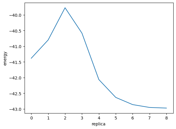
Let’s look at the results. The Notebook environment is also suitable for the graphical visualization of numerical data. Below is a visualization of an energy profile using matplotlib.
You can see the energy going up once and then going down in the reaction. The energy difference between the point of maximum energy (transition state) and each of the left and right stable points corresponds to the activation energy.
[7]:
energies = np.array([image.get_total_energy() for image in images])

fig = plt.figure()
ax = fig.add_subplot(1, 1, 1)
ax.plot(energies)
ax.set_xlabel("replica")
ax.set_ylabel("energy")
fig.show()
The activation energy can be calculated as follows.
Here, the activation energy in the forward reaction X→Y is denoted as E_act_forward, and reverse reaction Y→X is denoted as E_act_backward.
[8]:
# Transition state takes maximum energy in the reaction path
ts_index = np.argmax(energies)

E_act_forward = energies[ts_index] - energies[0]
E_act_backward = energies[ts_index] - energies[-1]

print(f"ts_index       = {ts_index}")
print(f"E_act_forward  = {E_act_forward:.2f} eV")
print(f"E_act_backward = {E_act_backward:.2f} eV")
ts_index       = 3
E_act_forward  = 1.93 eV
E_act_backward = 3.48 eV
You can visualize the structure in the Notebook as well, or you can save the image as a file. Let’s have a try.
The results are output as a trajectories rather than a single structure since it is NEB calculation. Let’s save it as an animated GIF using ASE.
[9]:
fig = plt.figure(facecolor="white")
ax = fig.add_subplot()
ase.io.write(
    "output/curtius_NEB.gif",
    images,
    format="gif",
    ax=ax
)
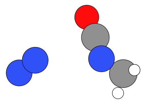
You can see a static image of the final structure above, but if you double-click on “curtius_NEB.gif” in the file viewer on the left, you can directly see the animated GIF.
If the calculations are successful, you will see the following animated GIFs.
[10]:
Image("output/curtius_NEB.gif", format="gif")
[10]:
<IPython.core.display.Image object>
Finally, let’s compare how the NEB method changed the reaction path before and after optimization.
Call the neb.interpolate() function and compare the energy of the candidate structure interpolated_images of the reaction pathway before FIRE opt, and images after optimization by the NEB.
[11]:
_images = [react.copy()]
_images += [react.copy() for i in range (7)]
_images += [prod.copy()]
for image in _images:
    estimator = Estimator()
    calculator = ASECalculator(estimator)
    image.calc = calculator
neb = NEB(_images, k=0.1, climb=True, allow_shared_calculator=False, parallel=True)
neb.interpolate()
interpolated_images = _images
/tmp/ipykernel_38727/4187733795.py:8: FutureWarning: Please import NEB from ase.mep, not ase.neb.
  neb = NEB(_images, k=0.1, climb=True, allow_shared_calculator=False, parallel=True)
[12]:
initial_energies = [image.get_total_energy() for image in interpolated_images]
opt_energies = [image.get_total_energy() for image in images]

fig = plt.figure()
ax = fig.add_subplot(1, 1, 1)
ax.plot(initial_energies, label="neb interpolated", color="red")
ax.plot(energies, label="after neb opt")
ax.set_xlabel("replica")
ax.set_ylabel("energy")
ax.legend()
fig.show()
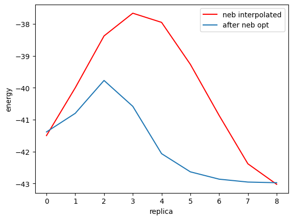
As can be seen from the above figure, NEB method has led to the discovery of a pathway with lower activation energy than the candidate reaction pathway (red line), i.e., a pathway with lower transition state energy (blue line).
[Column] Comparison of reaction pathway analysis methods and molecular dynamics
In this section, the reaction pathway was explored using the NEB method, which specifies the starting and ending states.
Molecular dynamics (MD) methods, described in the next chapter, can follow the time evolution of atoms. So, what about running the MD simulation until the chemical reaction occurs naturally? There are examples where activation energies can be analyzed by MD as well. The diffusion phenomenon of the Li ion is such an example.
However, reaction time is a challenging issue in general. Reactions are rare events. As you can see from the Arrhenius equation, it is a phenomenon whose frequency of occurrence changes exponentially with respect to the activation energy \(E_a\).
Therefore, MD can see the reaction if the activation energy is very low. However, if the activation energy becomes higher, the reaction does not occur in the time scale that MD can handle (~ns) and cannot be detected efficiently. Futhermore, if the activation energy is even higher, it will be a phenomenon that does not occur even in the real world.
For reference, let us look at the relationship between activation energy and the likelihood of a phenomenon. At 300 K, which is about room temperature, the value of \(k_B T\), which is the denominator inside the exponential function of the Arrhenius equation, is roughly 0.026 eV. This means that the occurrence probablilty of a phenomenon with 1 eV higher activation energy is reduced by a factor of \(\exp\left(-1/0.026\right)\), or \(2\times10^{-17}\). Even considering the difference between macroscale and atomic scale, this is still a large differencet and the reaction can be regarded as a rare event. Similarly, \(k_B T\) is 0.086 eV and 0.172 eV at 1000 K and 2000 K, respectively. It means that the likelihood of a phenomenon with 1 eV higher activation energy is about \(9 \times10^{-6}\) and \(0.003\) times lower, respectively. This is significantly larger than the value at 300 K, and can be regarded as a frequently occurring phenomenon on the macroscopic scale. In general, the occurrence probability of the phenomenon is very sensitive to the activation energy and temperature. By using reaction path analysis such as the NEB method, it is possible to efficiently analyze such rare events across exponential scales.
[13]:
from ase.units import kB
from math import exp

for T in [300, 1000, 2000]:
    kBT = kB * T
    ratio = exp(-1 / (kBT))

    print(f"----- T = {T} K -----")
    print(f"kB T : {kBT:.3f}")
    print(f"ratio: {ratio:.2e}")
----- T = 300 K -----
kB T : 0.026
ratio: 1.59e-17
----- T = 1000 K -----
kB T : 0.086
ratio: 9.12e-06
----- T = 2000 K -----
kB T : 0.172
ratio: 3.02e-03
In this sense, it may be possible to efficiently explore reactions that are difficult to see with MD by using the NEB method.
In addition, several approaches for reaction path searching are described below.
Approach | Characteristic | Methods |
|---|---|---|
Reaction pathway search for a specific reaction pathway | A method to find the minimum energy path (MEP) in a neighborhood starting from a path connecting two stable structures. Although the MEP and the corresponding transition state can be found with relatively low computational cost, the results strongly depend on the reaction path assumed before the search because it is local search method. | NEB, String method etc. |
Reaction path search without assuming reaction paths in advance | A method to find one or more reaction pathways without a priori assumptions about reaction pathways or post-reaction structures. In addition to the standard method of MD, there are other methods such as metadynamics, which aims to efficiently search for energy surfaces, and a method that uses information on local energy surfaces to search (ADDF). | MD, metadynamics, ADDF etc. |
Reference
The following references may be useful to those who would like to study further.