Molecular Dynamics simulation
TL;DR
MD simulations follow the equations of motion of classical mechanics, and the time evolution of the positions and velocities of all atoms can be observed.
The upper limit is generally a few dozen ns due to the time scale limitation. If a phenomenon does not occur within that time, it is necessary to consider a different calculation method.
In MD simulations, there are various states (ensembles) depending on the state to be reproduced, and the simplest ensemble is called the NVE ensemble.
In the NVE ensemble, the total energy conservation law holds, and the time step must be set appropriately in terms of calculation accuracy and calculation time.
In this chapter, you will learn about Molecular dynamics (MD), which simulates the time evolution of a system.
MD simulation explicitly deals with the time evolution of the trajectories of individual atoms. It is a method that calculates the coordinates and velocities of the target atoms sequentially by integrating the equations of motion of classical mechanics. This calculation method itself is a theory independent of models of forces and energies acting between atoms, and has long been used in the field of molecular simulation. Therefore, for the theoretical background and examples, please refer to the existing books and references (for example, [1-3]). The purpose of this tutorial is to acquire the pracitical knowledge necessary to perform these calculations using Matlantis.
Let’s take a look at what can be observed in an MD simulation by running an example.
Preliminary setup - Installation of required libraries
Through this chapter, we sometimes use ASAP3-EMT, which is a classical force field easily accessible on ASE. Since it is a classical force field, its accuracy and application are limited, but it is so simple and fast that very useful to demonstrate important points in this tutorial without much hustle and frustration. The elements available in ASAP3-EMT are limited to Ni, Cu, Pd, Ag, Pt, Au and their alloys. The installation procedure is as follows.
[1]:
!pip install --upgrade asap3
Looking in indexes: https://pypi.org/simple, http://pypi.artifact.svc:8080/simple
Collecting asap3
  Downloading asap3-3.13.7.tar.gz (855 kB)
     ━━━━━━━━━━━━━━━━━━━━━━━━━━━━━━━━━━━━━━ 855.8/855.8 kB 65.4 MB/s eta 0:00:00
  Installing build dependencies ... one
  Getting requirements to build wheel ... done
  Installing backend dependencies ... one
  Preparing metadata (pyproject.toml) ... done
Requirement already satisfied: ase>=3.23.0 in /home/jovyan/.py311/lib/python3.11/site-packages (from asap3) (3.25.0)
Requirement already satisfied: numpy>=1.19.5 in /home/jovyan/.py311/lib/python3.11/site-packages (from ase>=3.23.0->asap3) (1.26.4)
Requirement already satisfied: scipy>=1.6.0 in /home/jovyan/.py311/lib/python3.11/site-packages (from ase>=3.23.0->asap3) (1.15.3)
Requirement already satisfied: matplotlib>=3.3.4 in /home/jovyan/.py311/lib/python3.11/site-packages (from ase>=3.23.0->asap3) (3.10.3)
Requirement already satisfied: contourpy>=1.0.1 in /home/jovyan/.py311/lib/python3.11/site-packages (from matplotlib>=3.3.4->ase>=3.23.0->asap3) (1.3.2)
Requirement already satisfied: cycler>=0.10 in /home/jovyan/.py311/lib/python3.11/site-packages (from matplotlib>=3.3.4->ase>=3.23.0->asap3) (0.12.1)
Requirement already satisfied: fonttools>=4.22.0 in /home/jovyan/.py311/lib/python3.11/site-packages (from matplotlib>=3.3.4->ase>=3.23.0->asap3) (4.58.2)
Requirement already satisfied: kiwisolver>=1.3.1 in /home/jovyan/.py311/lib/python3.11/site-packages (from matplotlib>=3.3.4->ase>=3.23.0->asap3) (1.4.8)
Requirement already satisfied: packaging>=20.0 in /home/jovyan/.py311/lib/python3.11/site-packages (from matplotlib>=3.3.4->ase>=3.23.0->asap3) (25.0)
Requirement already satisfied: pillow>=8 in /home/jovyan/.py311/lib/python3.11/site-packages (from matplotlib>=3.3.4->ase>=3.23.0->asap3) (11.2.1)
Requirement already satisfied: pyparsing>=2.3.1 in /home/jovyan/.py311/lib/python3.11/site-packages (from matplotlib>=3.3.4->ase>=3.23.0->asap3) (3.2.3)
Requirement already satisfied: python-dateutil>=2.7 in /home/jovyan/.py311/lib/python3.11/site-packages (from matplotlib>=3.3.4->ase>=3.23.0->asap3) (2.9.0.post0)
Requirement already satisfied: six>=1.5 in /home/jovyan/.py311/lib/python3.11/site-packages (from python-dateutil>=2.7->matplotlib>=3.3.4->ase>=3.23.0->asap3) (1.17.0)
Building wheels for collected packages: asap3
done
  Created wheel for asap3: filename=asap3-3.13.7-cp311-cp311-linux_x86_64.whl size=4461488 sha256=8ef68bdc4c47a62e592d5d40598d3921480daf8f34de9a6d3b63d718ff1ec1b7
  Stored in directory: /home/jovyan/.cache/pip/wheels/d1/8c/80/5aa8169f1b9773bb685620a4ce577adcd238f95b106ce06013
Successfully built asap3
Installing collected packages: asap3
Successfully installed asap3-3.13.7

[notice] A new release of pip is available: 24.0 -> 25.1.1
[notice] To update, run: pip install --upgrade pip
For details about ASAP3-EMT, please refer ASAP official page.
What can MD simulation do?
In the following example, the MD simulation reproduces the molten state of a metallic Al structure. As everyone knows, aluminum is one of the most common metal in both commertial and industrial sectors. Its properties are well known. It has a melting point of 660.3 °C (933.45 K) and the face-centered cubic (fcc) phase is stable over a wide temperature range under ambient pressure. The following shows the process of melting the fcc-Al structure by heating it to an initial temperature of 1600 K. The calculation time is 100 psec.
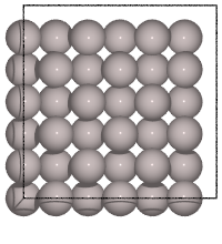
Fig6-1a. Melting of fcc-Al in NVE ensemble starting at 1600 K
(File: ../input/ch6/6-1_fcc-Al_NVE_1600Kstart.traj)
The Al atoms are initially arranged in a clean fcc crystal structure, but the structure is gradually disrupted and the atoms gradually diffuse out of the simulation cell as the calculation proceeds. In this way, MD simulations allow us to observe in detail the actual trajectories of the atoms as they evolve over time.
Simulation of aluminum melting
Below is a sample code of the MD simulation used to reproduce the melting process of fcc-Al described above. The ASAP3 EMT force field is used to speed up the calculation. (To use this force field in your python environment, you must first install the asap3 package by running pip install asap3.) The following calculation runs for 100 psec MD and takes only a few tens of seconds to complete.
[2]:
%%time
import os
from asap3 import EMT
calculator = EMT()

from ase.build import bulk
from ase.md.velocitydistribution import MaxwellBoltzmannDistribution,Stationary
from ase.md.verlet import VelocityVerlet
from ase.md import MDLogger
from ase import units
from time import perf_counter
import numpy as np

# Set up a fcc-Al crystal
atoms = bulk("Al","fcc",a=4.3,cubic=True)
atoms.pbc = True
atoms *= 3
print("atoms = ",atoms)

# Set calculator (EMT in this case)
atoms.calc = calculator

# input parameters
time_step    = 1.0      # MD step size in fsec
temperature  = 1600     # Temperature in Kelvin
num_md_steps = 100000   # Total number of MD steps
num_interval = 1000     # Print out interval for .log and .traj

# Set the momenta corresponding to the given "temperature"
MaxwellBoltzmannDistribution(atoms, temperature_K=temperature,force_temp=True)
Stationary(atoms)  # Set zero total momentum to avoid drifting

# Set output filenames
output_filename = "./output/ch6/liquid-Al_NVE_1.0fs_test"
log_filename = output_filename + ".log"
print("log_filename = ",log_filename)
traj_filename = output_filename + ".traj"
print("traj_filename = ",traj_filename)

# Remove old files if they exist
if os.path.exists(log_filename): os.remove(log_filename)
if os.path.exists(traj_filename): os.remove(traj_filename)

# Define the MD dynamics class object
dyn = VelocityVerlet(atoms,
                     time_step * units.fs,
                     trajectory = traj_filename,
                     loginterval=num_interval
                    )

# Print statements
def print_dyn():
    imd = dyn.get_number_of_steps()
    time_md = time_step*imd
    etot  = atoms.get_total_energy()
    ekin  = atoms.get_kinetic_energy()
    epot  = atoms.get_potential_energy()
    temp_K = atoms.get_temperature()
    print(f"   {imd: >3}     {etot:.9f}     {ekin:.9f}    {epot:.9f}   {temp_K:.2f}")

dyn.attach(print_dyn, interval=num_interval)

# Set MD logger
dyn.attach(MDLogger(dyn, atoms, log_filename, header=True, stress=False,peratom=False, mode="w"), interval=num_interval)

# Now run MD simulation
print(f"\n    imd     Etot(eV)    Ekin(eV)    Epot(eV)    T(K)")
dyn.run(num_md_steps)

print("\nNormal termination of the MD run!")
atoms =  Atoms(symbols='Al108', pbc=True, cell=[12.899999999999999, 12.899999999999999, 12.899999999999999])
log_filename =  ./output/ch6/liquid-Al_NVE_1.0fs_test.log
traj_filename =  ./output/ch6/liquid-Al_NVE_1.0fs_test.traj

    imd     Etot(eV)    Ekin(eV)    Epot(eV)    T(K)
     0     32.139701294     22.336120234    9.803581060   1600.00
   1000     32.144722159     9.393665122    22.751057037   672.90
   2000     32.144501700     10.379779872    21.764721828   743.53
   3000     32.144318649     10.246193775    21.898124875   733.96
   4000     32.144092145     11.057828314    21.086263831   792.10
   5000     32.144046250     11.951114265    20.192931985   856.09
   6000     32.144260378     10.923214025    21.221046353   782.46
   7000     32.144403860     10.881528388    21.262875472   779.47
   8000     32.144603170     10.966654516    21.177948654   785.57
   9000     32.144375218     11.119079419    21.025295799   796.49
   10000     32.144222322     11.189498687    20.954723635   801.54
   11000     32.144440573     9.685355360    22.459085213   693.79
   12000     32.144344847     10.762266046    21.382078801   770.93
   13000     32.144479122     8.902966113    23.241513009   637.74
   14000     32.144045468     11.006792340    21.137253128   788.45
   15000     32.144403754     10.902851629    21.241552125   781.00
   16000     32.144707168     9.021035461    23.123671707   646.20
   17000     32.144642186     10.023978285    22.120663901   718.05
   18000     32.144529839     10.291094693    21.853435146   737.18
   19000     32.144050744     11.312184244    20.831866500   810.32
   20000     32.144890930     9.067681632    23.077209298   649.54
   21000     32.143962314     11.384761628    20.759200686   815.52
   22000     32.144291661     11.076124249    21.068167412   793.41
   23000     32.144432732     10.505241125    21.639191607   752.52
   24000     32.144434143     9.677110695    22.467323448   693.20
   25000     32.144411792     10.096105345    22.048306447   723.21
   26000     32.144418684     10.314244415    21.830174269   738.84
   27000     32.144056137     10.819549400    21.324506737   775.04
   28000     32.144136380     10.282863144    21.861273236   736.59
   29000     32.144064247     10.603706988    21.540357259   759.57
   30000     32.144142785     10.559098906    21.585043879   756.38
   31000     32.144361966     9.657395222    22.486966744   691.79
   32000     32.144754870     8.707546903    23.437207967   623.75
   33000     32.144403555     10.326549807    21.817853748   739.72
   34000     32.143748162     11.951159073    20.192589088   856.10
   35000     32.144315603     10.100633141    22.043682462   723.54
   36000     32.144494671     9.299422264    22.845072408   666.14
   37000     32.144459312     10.264518196    21.879941116   735.28
   38000     32.144381071     10.328971396    21.815409675   739.89
   39000     32.143938348     10.560093761    21.583844587   756.45
   40000     32.144102210     10.942980034    21.201122176   783.88
   41000     32.144304063     9.758359111    22.385944952   699.02
   42000     32.144112774     10.411570083    21.732542691   745.81
   43000     32.144261663     11.015808525    21.128453137   789.09
   44000     32.143624324     11.206493107    20.937131217   802.75
   45000     32.143866741     10.944182507    21.199684234   783.96
   46000     32.144367770     9.874633405    22.269734364   707.35
   47000     32.143616353     11.287305027    20.856311326   808.54
   48000     32.144377245     10.154501900    21.989875345   727.40
   49000     32.144159709     10.059211532    22.084948176   720.57
   50000     32.144028665     9.486133089    22.657895576   679.52
   51000     32.143870407     10.461223944    21.682646463   749.37
   52000     32.144010351     11.677881834    20.466128517   836.52
   53000     32.143902994     11.086181772    21.057721222   794.13
   54000     32.144209243     10.877133213    21.267076030   779.16
   55000     32.143866159     11.672773150    20.471093009   836.15
   56000     32.144245550     10.188169764    21.956075786   729.81
   57000     32.144065429     10.540759442    21.603305987   755.06
   58000     32.144047181     11.236293826    20.907753356   804.89
   59000     32.144231273     10.845868548    21.298362725   776.92
   60000     32.144175394     10.095420061    22.048755333   723.16
   61000     32.144210124     10.751451533    21.392758591   770.16
   62000     32.144358234     9.409524372    22.734833861   674.03
   63000     32.144063044     10.947444309    21.196618735   784.20
   64000     32.144231053     11.017702487    21.126528566   789.23
   65000     32.144695236     9.546443148    22.598252088   683.84
   66000     32.144162224     11.276822936    20.867339288   807.79
   67000     32.144488062     10.519866599    21.624621463   753.57
   68000     32.144557555     10.129716371    22.014841184   725.62
   69000     32.144450322     10.284807689    21.859642633   736.73
   70000     32.144447181     10.400649435    21.743797746   745.03
   71000     32.144632289     9.627578409    22.517053880   689.65
   72000     32.144341422     10.961964783    21.182376639   785.24
   73000     32.144545573     10.711859413    21.432686160   767.32
   74000     32.144810591     9.861638540    22.283172051   706.42
   75000     32.144743025     10.142373359    22.002369665   726.53
   76000     32.144666166     10.330929323    21.813736843   740.03
   77000     32.145018460     9.962101343    22.182917118   713.61
   78000     32.144948334     10.163190408    21.981757925   728.02
   79000     32.144724224     10.841427576    21.303296648   776.60
   80000     32.144567401     10.946160891    21.198406510   784.10
   81000     32.144693558     10.170510668    21.974182891   728.54
   82000     32.144802089     9.862497743    22.282304346   706.48
   83000     32.145176925     9.213573320    22.931603605   659.99
   84000     32.145220296     9.216727852    22.928492444   660.22
   85000     32.145225359     8.782294025    23.362931334   629.10
   86000     32.145009261     7.957304052    24.187705209   570.00
   87000     32.144947628     8.411435060    23.733512568   602.54
   88000     32.144898967     8.540565949    23.604333018   611.79
   89000     32.145000371     8.278721461    23.866278910   593.03
   90000     32.144782624     8.383947198    23.760835427   600.57
   91000     32.145227363     8.091000385    24.054226978   579.58
   92000     32.144911313     8.987582334    23.157328979   643.81
   93000     32.145250110     7.310771383    24.834478726   523.69
   94000     32.144846879     9.663598769    22.481248111   692.23
   95000     32.145210301     8.115149170    24.030061131   581.31
   96000     32.144906799     8.290101213    23.854805586   593.84
   97000     32.144800583     7.827986525    24.316814058   560.74
   98000     32.145024360     8.451294407    23.693729953   605.39
   99000     32.144819857     8.631967805    23.512852051   618.33
   100000     32.145028766     8.010498131    24.134530635   573.81

Normal termination of the MD run!
CPU times: user 25.6 s, sys: 203 ms, total: 25.8 s
Wall time: 25.6 s
The flow of the program can be understood by looking at the comments in the script, but the important points are explained here.
(1) Initial velocity distribution
Once the structure has been created and the calculation parameters have been set, the initial velocity of each atom is given by a velocity distribution corresponding to the specified temperature Maxwell-Boltzmann distribution. This is done using the MaxwellBoltzmannDistribution in above code. Since the initial velocity given by this method has arbitrary momentum of the whole system, there is a possibility that the
whole system may drift. Therefore, after giving the initial velocity by MaxwellBoltzmannDistribution, we set the momentum of the entire system to zero by the Stationary method and fix the coordinates of the center of mass. This is important not only for the NVE case, but also for simulations involving temperature and pressure control that will follow.
(2) Execute MD
This time, MD by Verlet integration is executed using the class VelocityVerlet. MD is actually executed at dyn.run(num_md_steps). In this time, time_step=1.0 (time width of 1fs = \(1 \times 10^{-15}\) sec per step) is used to execute num_md_steps=100000 steps.
(3) Recording of calculation results
The script has a method named print_dyn that prints energy and temperature values to standard output (output on a notebook). There is another class, MDLogger, which outputs energy, temperature, and stress information in a specified log file. You can define your own class to output the calculation results to a file, but the default logger provides the necessary information for most applications, so it is recommended to utilize it.
After MD is executed, the trajectory can be visualized as follows.
[3]:
from ase.io import Trajectory
from pfcc_extras.visualize.view import view_ngl


traj = Trajectory(traj_filename)
view_ngl(traj)
[3]:
[4]:
from pfcc_extras.visualize.povray import traj_to_apng
from IPython.display import Image


traj_to_apng(traj, f"output/Fig6-1_fcc-Al_NVE_1600Kstart.png", rotation="0x,0y,0z", clean=True, n_jobs=16)

# See Fig6-1a
#Image(url="output/Fig6-1_fcc-Al_NVE_1600Kstart.png")
[Parallel(n_jobs=16)]: Using backend ThreadingBackend with 16 concurrent workers.
[Parallel(n_jobs=16)]: Done  18 tasks      | elapsed:   12.8s
[Parallel(n_jobs=16)]: Done 101 out of 101 | elapsed:   41.7s finished
History of physical properties in NVE ensembles
Since the velocity (i.e., momentum) of each atom is known, the history of the various energies of the system can be followed. For example, here are the time profiles of total energy (Tot.E.), potential energy (P.E.), kinetic energy (K.E.), and temperature (Temp.) for the melting of fcc-Al.
[5]:
import pandas as pd

df = pd.read_csv(log_filename, delim_whitespace=True)
df
/tmp/ipykernel_50921/510401485.py:3: FutureWarning: The 'delim_whitespace' keyword in pd.read_csv is deprecated and will be removed in a future version. Use ``sep='\s+'`` instead
  df = pd.read_csv(log_filename, delim_whitespace=True)
[5]:
| Time[ps] | Etot[eV] | Epot[eV] | Ekin[eV] | T[K] | |
|---|---|---|---|---|---|
| 0 | 0.0 | 32.140 | 9.804 | 22.336 | 1600.0 |
| 1 | 1.0 | 32.145 | 22.751 | 9.394 | 672.9 |
| 2 | 2.0 | 32.145 | 21.765 | 10.380 | 743.5 |
| 3 | 3.0 | 32.144 | 21.898 | 10.246 | 734.0 |
| 4 | 4.0 | 32.144 | 21.086 | 11.058 | 792.1 |
| ... | ... | ... | ... | ... | ... |
| 96 | 96.0 | 32.145 | 23.855 | 8.290 | 593.8 |
| 97 | 97.0 | 32.145 | 24.317 | 7.828 | 560.7 |
| 98 | 98.0 | 32.145 | 23.694 | 8.451 | 605.4 |
| 99 | 99.0 | 32.145 | 23.513 | 8.632 | 618.3 |
| 100 | 100.0 | 32.145 | 24.135 | 8.010 | 573.8 |
101 rows × 5 columns
[6]:
import numpy as np
import matplotlib.pyplot as plt


fig = plt.figure(figsize=(10, 5))

#color = 'tab:grey'
ax1 = fig.add_subplot(4, 1, 1)
ax1.set_xticklabels([])
ax1.set_ylabel('Tot E (eV)')
ax1.set_ylim([31.,33.])
ax1.plot(df["Time[ps]"], df["Etot[eV]"], color="blue",alpha=0.5)

ax2 = fig.add_subplot(4, 1, 2)
ax2.set_xticklabels([])
ax2.set_ylabel('P.E. (eV)')
ax2.plot(df["Time[ps]"], df["Epot[eV]"], color="green",alpha=0.5)

ax3 = fig.add_subplot(4, 1, 3)
ax3.set_xticklabels([])
ax3.set_ylabel('K.E. (eV)')
ax3.plot(df["Time[ps]"], df["Ekin[eV]"], color="orange",alpha=0.5)

ax4 = fig.add_subplot(4, 1, 4)
ax4.set_xlabel('time (ps)')
ax4.set_ylabel('Temp. (K)')
ax4.plot(df["Time[ps]"], df["T[K]"], color="red",alpha=0.5)
ax4.set_ylim([500., 1700])

fig.suptitle("Fig.6-1b. Time evolution of total, potential, and kinetic energies, and temperature.", y=0)

#plt.savefig("6-1_liquid-Al_NVE_1.0fs_test_E_vs_t.png")  # <- Use if saving to an image file is desired
plt.show()
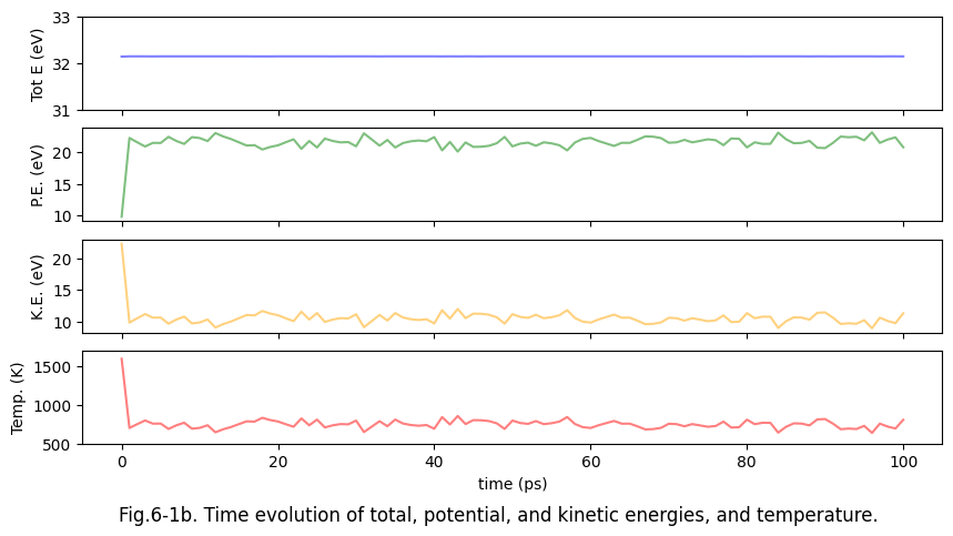
As mentioned in section 1-5, the total energy \(E\) of a system is expressed by the kinetic energy \(K\) and the potential energy \(V\).
Of these, the kinetic energy \(K\) of a system can be calculated as follows, using the formula from classical mechanics.
where \(m_i, \mathbf{v}_i, \mathbf{p}_i\) are the mass, velocity and momentum (\(\mathbf{p}=m\mathbf{v}\)) of each atom respectively. Here, the temperature and kinetic energy of the system are synonymous and are defined by the following relationship.
In this case, the initial temperature is set to 1600 K, and the system evolves naturally in time according to the equations of motion of classical mechanics. Since there is no external force, the energy conservation law is obeyed and the total energy is kept constant within the numerical error. The temperature decreases fairly quickly, and the kinetic and potential energies follows the equipartition theorem, and the temperature eventually settles to about half the initial temperature. This is how matter actually behaves in nature, and the simplest MD simulations such as this one reproduce such a situation. The distribution of states of such a system is shown in NVE Ensemble. (or microcanonical ensemble, where N stands for the number of atoms, V for the volume, and E for the total energy being constant.) The ensemble here refers to the distribution of states of system in the concept of statistical mechanics.
MD simulation parameters in NVE ensemble
In the MD simulation of the NVE ensemble described above, you need to set the calculation conditions like initial temperature and calculation time. In addition, we also need to set the MD time step as a relatively non-trivial parameter. How should this MD time step be set?
The answer depends on the accuracy of the calculation you are looking for: the NVE ensemble solves the classical equations of motion, which are second-order ordinary differential equations, and the accuracy of this integration process is determined by the size of the time step. (more details on integration methods are given at the end of this section). Let us see how the total energy changes when the time step is changed. Let us assume that the computation time is 1 nsec. (This is a time scale often used in classical MD.)
Fig.6-1c. Time evolution of the total energy with respect to time step size.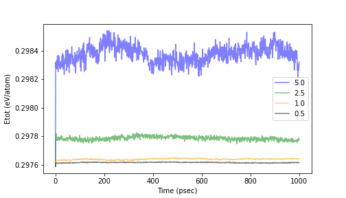
The above figure shows the calculation results when the time step is varied from 0.5 to 5.0 fsec. It can be seen that the total energy, which should be constant, has a large deviation with time evolution when the time step is large.
To check the time dependence of the total energy, run the above MD simulation script with different time_step arguments and compare the energy profiles as an excercise. For visualization, please refer to the visualization code shown in Fig. 6-1b above.
Varying the MD time step from the above calculations and plotting the RMSE obtained from the total energy fluctuations on the horizontal axis for the time step and the vertical axis for the total energy fluctuations, the results are shown below.
Fig.6-1d. Total energy ERMSE as a function of MD step size.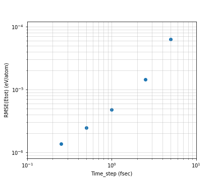
The vertical axis is the energy per atom, the plots can be seen to be roughly linear in a log-log plot. The energy per atom varies from 1.2e-6 eV at 0.25 fs to 6e-5 fs at 5.0 fs. In this case, the number of atoms is 108, so we can confirm that the entire system can vary from 1e-4 eV to 1e-3 eV.
In terms of energy, assuming a time step of 1 fsec, an error of about 0.5 meV is expected for a 100 atom system for a 1 nsec simulation, and about 5 meV for a 1000 atom system. Of course, it depends on the physical properties you want to calculate, but for most calculations, this should be accurate enough. If the time step is set to 5 fsec to increase the calculation time, the error will increase by about one order of magnitude. When using MD calculations, it is necessary to keep in mind the degree of accuracy of these calculations.
Other ensembles and MD Simulations
At the end of this section, we will discuss MD simulation methods other than NVE ensembles.
MD simulations of NVE ensembles are simple and powerful, but they have many disadvantages when it comes to reproducing the phenomena we generally want to observe. The atoms in the cell is all the computation target in the NVE simulation, and there is no external world. However, the microscopic world we actually want to observe has an environment surrounding it. The temperature and pressure of the external environment will change the state of the system of interest, which cannot be reproduced within the scope of the NVE ensemble.
There are various state distributions such as canonical ensemble (NVT), isothermal-isobaric ensemble (NPT), etc. in statistical mechanics, and they can be utilized to perform calculations under specific conditions. In the following sections, you will learn how to perform calculations under these statistical ensembles.
Reference
[1] M.P. Allen and D.J. Tildesley, “Computer simulaiton of liquid”, 2nd Ed., Oxford University Press (2017) ISBN 978-0-19-880319-5. DOI:10.1093/oso/9780198803195.001.0001
[2] D. Frenkel and B. Smit “Understanding molecular simulation - from algorithms to applications”, 2nd Ed., Academic Press (2002) ISBN 978-0-12-267351-1. DOI:10.1016/B978-0-12-267351-1.X5000-7
[3] M.E. Tuckerman, “Statistical mechanics: Theory and molecular simulation”, Oxford University Press (2010) ISBN 978-0-19-852526-4. https://global.oup.com/academic/product/statistical-mechanics-9780198525264?q=Statistical%20mechanics:%20Theory%20and%20molecular%20simulation&cc=gb&lang=en#