NPT ensemble
TL;DR
In NPT-MD simulations, pressure and temperature are controlled and remain constant once the system reaches equilibrium. There are two common pressure control (barostat) methods available in ASE: the Parrinello-Rahman method and the Berendsen method.
Typical applications include simulations of thermal expansion, phase transitions, and pressurization of solids and fluids.
In the Parrinello-Rahman method, all degrees of freedom of the simulation cell are variable, and the control parameter (
pfactor) must be set appropriately.Berendsen barostat, like Berendsen thermostat, can control pressure efficiently for convergence; Berendsen barostat can be calculated in two modes: with fixed cell angles and independently variable cell lengths, or with fixed cell length ratios.
compressibilitymust be properly set as an input parameter.
In this section, we will discuss a method to create an equilibrium state in which both pressure and temperature are constant. The pressure control mechanism is generally referred to as barostat, and is used in conjunction with the thermostat method described in section 6-2 to generate a state distribution called an isothermal-isobaric ensemble (also known as NPT).
Phenomena that can be studied, in principle, in NPT-MD simulations include
Coefficient of thermal expansion of solids
Prediction of melting point
Phase transitions in solids
Density prediction of fluids (gases and liquids)
etc.
The reason why the word “in principle” is used is that the reproducibility of these phenomena depends greatly on the accuracy of the force field used in the calculation, and in particular, it is known to be very difficult to predict intermolecular forces and fluid states that depend on small energy differences. In this tutorial, we will learn about NPT-MD through the case study of solids, which are considered to have relatively high accuracy.
First, we will review the NPT-MD methods implemented in ASE that we will use in this tutorial. There are three types of implementations available for ASE
Class |
Ensemble |
Parameter |
thermostat |
barostat |
description |
|---|---|---|---|---|---|
NPT |
NPT |
time constant (\(\tau_t\)), pressure factor (pfactor) |
Nosé–Hoover |
Parrinello-Rahman |
セルの全All degrees of freedom of the cell are variable and controllable |
NPTBerendsen |
NPT |
\(\tau_t\),\(\tau_P\),\(\beta_T\) |
Berendsen |
Berendsen |
Cell shape is maintained and only volume changes |
InhomogeneousBerendsen |
NPT |
\(\tau_t\),\(\tau_P\),\(\beta_T\) |
Berendsen |
Berendsen |
Cell angles are preserved, but pressure anisotropy can be taken into account |
The second and third methods in the table are essentially the same Berendsen barostat. (The third method, InhomogeneousBerendsen, is not mentioned in the ASE manual, but is defined as a class within ASE along with NPTBerendsen.) Thus, there are only two methods available within the ASE framework: the Parrinello-Rahman method and the Berendsen method. The heat bath itself uses the methods described in section 6-2, so the characteristics of these heat bath methods should be carefully
considered.
Let us first look at the Parrinello-Rahman method, which has relatively high system flexibility and versatility.
Equations of motion for the Parrinello-Rahman method
The Parrinello-Rahman method is a so-called extended system calculation method, which assumes that the system under consideration is hypothetically connected to an external system of constant temperature and pressure, as in the Nosé-Hoover heat bath method. In this case, the equations of motion are written as follows (For details of the derivation, please refer to references [1-3]).
Besides the terms for the Nosé-Hoover heat bath, we have the pressure control time constant \(\tau_P\), the system center of mass \(R_o\), the target external pressure \(P_o\), and the simulation cell volume \(V\). The \(\eta\) is the variable for the pressure control degrees of freedom. \(\mathbf{h} = (\mathbf{a}, \mathbf{b}, \mathbf{c})\) and \(\mathbf{a},\mathbf{b},\mathbf{c}\) are cell vectors defining each edge of the simulation cell, respectively.
In addition to temperature \(T_o\) and pressure \(P_o\), there are two other values that the user must set in the above equation: \(\tau_T\) and \(\tau_P\). First, the case where \(\tau_T\) and \(\tau_P\) are simply set to random values is shown below. Here \(\tau_T\) is set to 20 fsec. Although \(\tau_P\) is not specified directly, the value called pfactor is \(\tau_P^2B\). The \(B\) refers to the bulk modulus, and this value must be calculated and
specified in advance. However, since the exact value of \(\tau_P\) itself is not known in advance, there is no way to specify pfactor. Also, the value of \(B\) cannot be calculated for anisotropic structures or when different types of materials coexist in the system. Therefore, we will set an approximate value of pfactor to examine the behavior of the barostat. As mentioned in the following example, at least for crystalline metal systems, a value on the order of about
10\(^6\) GPa\(\cdot\)fs\(^2\) to 10\(^7\) GPa\(\cdot\)fs\(^2\) seems to give good convergence and stability in the calculation. For other materials, it is recommended to play with the value of pfactor and check the behavior of the volume change as a preliminary study.
Calculation example: Coefficient of thermal expansion
Now, we will use the Nosé-Hoover thermostat and the Parrinello-Rahman barostat (ASE’s NPT class) to compute the coefficient of thermal expansion of a solid as an example. The system is equilibrated at temperatures of given increment, and the thermal expansion coefficient is calculated from the average value of the lattice constant at each temperature.
For simplicity, we will use fcc-Cu for this calculation. A sample script is shown below. The temperature is varied from 200 K to 1000 K in 100 K interval and the external pressure is set to 1 bar. The structure is fcc-Cu extended to 3x3x3 unit cells with 108 atoms. In the example, the ASAP3-EMT force field is used for speed, but the same scheme can be used with PFP. The time step size is set to 1 fs, and the 20 ps simulation is found to be sufficient to reach equilibrium.
[1]:
import ase
from ase.build import bulk
from ase.md.velocitydistribution import MaxwellBoltzmannDistribution,Stationary
from ase.md.npt import NPT
from ase.md import MDLogger
from ase import units
from time import perf_counter

calc_type = "EMT"
# calc_type = "PFP"

if calc_type == "EMT":
    # ASAP3-EMT calculator
    from asap3 import EMT
    calculator = EMT()
elif calc_type == "PFP":
    # PFP calculator
    from pfp_api_client.pfp.estimator import Estimator, EstimatorCalcMode
    from pfp_api_client.pfp.calculators.ase_calculator import ASECalculator
    estimator = Estimator(calc_mode=EstimatorCalcMode.PBE, model_version="v8.0.0")
    calculator = ASECalculator(estimator)
else:
    raise ValueError(f"Wrong calc_type = {calc_type}!")


# Set up a crystal
atoms_in = bulk("Cu",cubic=True)
atoms_in *= 3
atoms_in.pbc = True
print("atoms_in = ",atoms_in)

# input parameters
time_step    = 1.0    # fsec
#temperature = 300    # Kelvin
num_md_steps = 20000
num_interval = 10

sigma   = 1.0     # External pressure in bar
ttime   = 20.0    # Time constant in fs
pfactor = 2e6     # Barostat parameter in GPa
temperature_list = [200,300,400,500,600,700,800,900,1000]

# Print statements
def print_dyn():
    imd = dyn.get_number_of_steps()
    etot  = atoms.get_total_energy()
    temp_K = atoms.get_temperature()
    stress = atoms.get_stress(include_ideal_gas=True)/units.GPa
    stress_ave = (stress[0]+stress[1]+stress[2])/3.0
    elapsed_time = perf_counter() - start_time
    print(f"  {imd: >3}   {etot:.3f}    {temp_K:.2f}    {stress_ave:.2f}  {stress[0]:.2f}  {stress[1]:.2f}  {stress[2]:.2f}  {stress[3]:.2f}  {stress[4]:.2f}  {stress[5]:.2f}    {elapsed_time:.3f}")


# run MD
for i,temperature in enumerate(temperature_list):
    print("i,temperature = ",i,temperature)

    print(f"sigma = {sigma:.1e} bar")
    print(f"ttime = {ttime:.3f} fs")
    print(f"pfactor = {pfactor:.3f} GPa*fs^2")

    temperature_str = str(int(temperature)).zfill(4)
    output_filename = f"./output/ch6/fcc-Cu_3x3x3_NPT_{calc_type}_{temperature_str}K"
    log_filename = output_filename + ".log"
    traj_filename = output_filename + ".traj"
    print("log_filename = ",log_filename)
    print("traj_filename = ",traj_filename)

    atoms = atoms_in.copy()
    atoms.calc = calculator

    # Set the momenta corresponding to T=300K
    MaxwellBoltzmannDistribution(atoms, temperature_K=temperature,force_temp=True)
    Stationary(atoms)

    dyn = NPT(atoms,
          time_step*units.fs,
          temperature_K = temperature,
          externalstress = sigma*units.bar,
          ttime = ttime*units.fs,
          pfactor = pfactor*units.GPa*(units.fs**2),
          logfile = log_filename,
          trajectory = traj_filename,
          loginterval=num_interval
          )

    print_interval = 1000 if calc_type == "EMT" else num_interval
    dyn.attach(print_dyn, interval=print_interval)
    dyn.attach(MDLogger(dyn, atoms, log_filename, header=True, stress=True, peratom=True, mode="a"), interval=num_interval)

    # Now run the dynamics
    start_time = perf_counter()
    print(f"    imd     Etot(eV)    T(K)    stress(mean,xx,yy,zz,yz,xz,xy)(GPa)  elapsed_time(sec)")
    dyn.run(num_md_steps)
atoms_in =  Atoms(symbols='Cu108', pbc=True, cell=[10.83, 10.83, 10.83])
i,temperature =  0 200
sigma = 1.0e+00 bar
ttime = 20.000 fs
pfactor = 2000000.000 GPa*fs^2
log_filename =  ./output/ch6/fcc-Cu_3x3x3_NPT_EMT_0200K.log
traj_filename =  ./output/ch6/fcc-Cu_3x3x3_NPT_EMT_0200K.traj
    imd     Etot(eV)    T(K)    stress(mean,xx,yy,zz,yz,xz,xy)(GPa)  elapsed_time(sec)
    0   2.727    200.00    1.64  1.62  1.66  1.63  -0.03  -0.00  0.04    0.004
  1000   3.257    138.10    0.86  0.84  0.84  0.88  0.17  0.17  0.21    1.304
  2000   4.444    192.41    0.77  0.61  0.92  0.79  0.29  0.27  -0.04    2.563
  3000   4.381    187.60    0.93  1.03  0.94  0.84  0.12  0.08  0.30    3.808
  4000   4.599    181.45    0.52  0.42  0.76  0.39  0.05  0.05  0.21    5.072
  5000   5.692    202.32    -0.38  -0.38  -0.35  -0.41  -0.06  0.56  0.25    6.414
  6000   6.109    220.68    -0.65  -0.74  -0.68  -0.52  -0.20  0.02  0.04    7.671
  7000   5.639    219.03    -0.15  0.01  -0.36  -0.10  0.04  0.15  -0.01    8.902
  8000   5.351    205.21    0.45  0.44  0.39  0.53  0.05  0.24  -0.04    10.165
  9000   5.376    174.50    0.22  0.05  0.42  0.18  0.18  0.15  -0.17    11.484
  10000   5.744    196.53    -0.33  -0.46  -0.25  -0.27  0.05  -0.02  0.09    12.785
  11000   5.523    230.52    -0.30  -0.31  -0.43  -0.17  -0.00  0.05  0.15    14.047
  12000   4.885    184.51    -0.11  -0.14  -0.08  -0.13  0.30  0.12  -0.05    15.302
  13000   5.545    213.75    0.18  0.34  0.14  0.06  0.55  -0.12  0.03    16.610
  14000   6.289    218.35    0.14  0.21  0.33  -0.12  0.33  0.25  0.12    17.857
  15000   5.202    205.62    0.44  0.28  0.56  0.48  0.39  -0.08  -0.00    19.133
  16000   5.704    211.51    -0.37  -0.55  -0.22  -0.34  0.05  -0.40  -0.18    20.411
  17000   5.178    184.93    -0.52  -0.41  -0.71  -0.45  0.04  -0.17  -0.10    21.694
  18000   5.410    192.98    -0.25  -0.03  -0.46  -0.27  0.08  -0.11  -0.26    22.949
  19000   6.283    234.67    0.13  0.31  -0.06  0.15  -0.06  -0.20  -0.16    24.195
  20000   5.147    180.81    0.62  0.69  0.56  0.60  -0.14  -0.20  -0.49    25.469
i,temperature =  1 300
sigma = 1.0e+00 bar
ttime = 20.000 fs
pfactor = 2000000.000 GPa*fs^2
log_filename =  ./output/ch6/fcc-Cu_3x3x3_NPT_EMT_0300K.log
traj_filename =  ./output/ch6/fcc-Cu_3x3x3_NPT_EMT_0300K.traj
    imd     Etot(eV)    T(K)    stress(mean,xx,yy,zz,yz,xz,xy)(GPa)  elapsed_time(sec)
    0   4.123    300.00    1.52  1.61  1.46  1.50  -0.01  -0.03  -0.01    0.002
  1000   7.039    294.54    0.62  0.76  0.50  0.62  -0.02  -0.11  -0.11    1.289
  2000   6.642    266.68    1.46  1.74  1.57  1.06  -0.25  0.02  0.05    2.559
  3000   7.757    288.57    1.48  1.52  1.57  1.34  -0.15  -0.16  0.39    3.823
  4000   8.489    291.95    0.31  0.34  -0.02  0.61  0.08  -0.08  0.58    5.096
  5000   8.163    265.87    -0.89  -1.07  -1.04  -0.57  0.11  0.19  0.65    6.381
  6000   8.944    336.60    -1.32  -1.24  -1.20  -1.53  0.20  0.60  0.37    7.666
  7000   7.524    257.73    -0.28  -0.18  -0.06  -0.62  -0.13  0.11  0.52    8.908
  8000   8.845    311.11    0.50  0.57  0.61  0.32  0.21  0.36  0.73    10.169
  9000   8.675    306.12    1.05  1.08  0.82  1.24  0.52  0.10  0.73    11.489
  10000   8.658    313.89    0.58  0.47  0.39  0.87  0.74  0.14  0.74    12.752
  11000   9.631    395.51    -0.49  -0.43  -0.62  -0.41  0.52  0.40  0.70    13.999
  12000   8.691    286.93    -1.19  -0.96  -1.09  -1.52  0.28  0.22  0.49    15.278
  13000   7.403    260.96    -0.60  -0.56  -0.29  -0.95  0.51  -0.03  0.44    16.553
  14000   9.016    325.97    -0.14  -0.04  -0.17  -0.21  0.54  -0.07  0.80    17.834
  15000   9.425    316.12    0.55  0.62  0.28  0.76  0.44  0.02  0.89    19.086
  16000   8.362    287.70    0.83  0.60  0.85  1.05  0.38  0.08  0.89    20.360
  17000   8.799    292.57    -0.21  -0.49  0.24  -0.37  -0.02  -0.38  0.91    21.664
  18000   8.024    293.51    -0.65  -0.50  -0.71  -0.73  -0.23  0.08  1.02    22.930
  19000   8.160    303.79    -0.84  -0.47  -1.30  -0.73  -0.11  -0.19  1.18    24.190
  20000   9.328    351.21    -0.45  -0.40  -0.89  -0.06  -0.17  -0.22  1.09    25.461
i,temperature =  2 400
sigma = 1.0e+00 bar
ttime = 20.000 fs
pfactor = 2000000.000 GPa*fs^2
log_filename =  ./output/ch6/fcc-Cu_3x3x3_NPT_EMT_0400K.log
traj_filename =  ./output/ch6/fcc-Cu_3x3x3_NPT_EMT_0400K.traj
    imd     Etot(eV)    T(K)    stress(mean,xx,yy,zz,yz,xz,xy)(GPa)  elapsed_time(sec)
    0   5.519    400.00    1.40  1.47  1.33  1.41  -0.07  0.04  -0.06    0.003
  1000   11.615    433.05    -1.87  -1.41  -2.02  -2.19  -0.34  -0.03  -0.12    1.265
  2000   12.383    419.09    -0.11  0.46  0.03  -0.82  -0.31  -0.01  0.22    2.529
  3000   11.877    413.81    2.05  2.38  2.37  1.39  -0.11  0.04  -0.28    3.805
  4000   11.944    409.88    2.15  1.89  2.46  2.11  0.18  -0.01  -0.21    5.076
  5000   11.040    381.69    0.96  0.81  0.82  1.26  0.10  -0.00  0.60    6.369
  6000   10.106    394.10    -0.40  -0.22  -1.01  0.04  -0.02  -0.30  0.23    7.647
  7000   10.675    424.80    -1.73  -1.60  -1.97  -1.60  -0.13  -0.82  0.54    8.945
  8000   11.052    382.51    -1.81  -1.64  -1.59  -2.21  -0.24  -0.54  -0.04    10.224
  9000   11.590    414.92    -0.36  -0.14  -0.16  -0.79  -0.56  -0.64  0.28    11.498
  10000   10.523    341.87    1.38  1.67  1.18  1.27  -0.14  -0.24  0.33    12.762
  11000   10.769    359.31    1.98  2.01  1.77  2.15  0.27  -0.08  0.19    14.014
  12000   11.827    390.91    0.78  0.84  0.67  0.81  0.17  -0.72  0.01    15.283
  13000   11.848    448.43    -0.54  -0.82  -0.11  -0.68  0.49  -0.85  0.76    16.570
  14000   10.131    371.62    -1.29  -1.31  -0.92  -1.64  -0.22  -0.86  0.65    17.851
  15000   10.884    413.01    -1.32  -1.05  -1.42  -1.49  0.33  -0.59  0.60    19.117
  16000   10.524    347.84    -0.50  -0.26  -1.03  -0.22  0.27  -1.27  0.16    20.391
  17000   12.336    410.07    0.30  0.30  0.49  0.11  0.38  -0.29  0.34    21.652
  18000   11.884    372.32    1.41  0.92  2.28  1.03  0.50  -0.44  0.32    22.936
  19000   11.505    398.81    1.77  1.47  2.62  1.22  -0.01  -0.95  0.20    24.188
  20000   11.140    403.94    0.67  0.88  0.21  0.92  -0.05  -0.59  -0.48    25.481
i,temperature =  3 500
sigma = 1.0e+00 bar
ttime = 20.000 fs
pfactor = 2000000.000 GPa*fs^2
log_filename =  ./output/ch6/fcc-Cu_3x3x3_NPT_EMT_0500K.log
traj_filename =  ./output/ch6/fcc-Cu_3x3x3_NPT_EMT_0500K.traj
    imd     Etot(eV)    T(K)    stress(mean,xx,yy,zz,yz,xz,xy)(GPa)  elapsed_time(sec)
    0   6.915    500.00    1.29  1.31  1.29  1.27  0.05  -0.06  -0.06    0.003
  1000   12.058    479.42    -1.63  -1.76  -1.58  -1.57  -0.08  0.32  0.65    1.308
  2000   12.707    510.71    0.12  -0.36  0.33  0.38  -0.04  0.75  -0.04    2.558
  3000   15.222    539.00    1.53  1.90  1.36  1.32  -0.24  0.64  0.21    3.825
  4000   14.956    487.91    3.19  3.80  2.80  2.96  -0.11  0.89  0.05    5.093
  5000   16.151    489.16    3.07  2.97  3.59  2.64  -0.13  0.75  0.43    6.351
  6000   15.795    561.85    2.81  2.43  3.07  2.93  -0.09  0.32  0.57    7.608
  7000   13.226    489.39    1.42  1.18  1.52  1.56  0.09  0.27  -0.35    8.856
  8000   13.933    547.11    -1.62  -1.45  -1.61  -1.79  0.01  0.47  -0.56    10.128
  9000   14.159    497.65    -3.89  -3.67  -3.95  -4.06  0.13  0.59  -0.26    11.450
  10000   13.296    480.78    -3.69  -3.94  -4.40  -2.74  0.40  0.33  -0.59    12.716
  11000   13.504    483.52    -1.88  -2.03  -1.77  -1.84  0.84  0.56  -0.95    13.992
  12000   13.670    457.77    0.13  0.35  0.23  -0.19  0.59  0.35  -0.08    15.287
  13000   15.112    553.76    1.80  2.25  2.06  1.09  -0.05  0.72  -0.22    16.557
  14000   16.743    627.12    2.40  2.63  2.49  2.08  -0.45  0.90  -0.51    17.804
  15000   15.498    497.26    1.54  1.58  0.95  2.11  -0.65  0.32  -0.69    19.082
  16000   15.301    539.67    0.45  0.58  0.41  0.37  -0.98  0.72  -0.48    20.359
  17000   13.511    481.97    -0.65  -0.70  -0.12  -1.12  -1.35  1.57  0.06    21.635
  18000   13.369    510.93    -1.23  -1.77  -1.05  -0.89  -1.19  0.50  -0.89    22.896
  19000   14.594    496.53    -1.81  -2.12  -1.74  -1.58  -0.90  0.74  -1.54    24.173
  20000   15.085    526.83    -0.78  -0.43  -1.62  -0.30  -0.67  0.92  -1.49    25.436
i,temperature =  4 600
sigma = 1.0e+00 bar
ttime = 20.000 fs
pfactor = 2000000.000 GPa*fs^2
log_filename =  ./output/ch6/fcc-Cu_3x3x3_NPT_EMT_0600K.log
traj_filename =  ./output/ch6/fcc-Cu_3x3x3_NPT_EMT_0600K.traj
    imd     Etot(eV)    T(K)    stress(mean,xx,yy,zz,yz,xz,xy)(GPa)  elapsed_time(sec)
    0   8.311    600.00    1.17  1.19  1.10  1.22  0.08  0.09  -0.13    0.002
  1000   16.715    639.49    -5.01  -5.06  -5.46  -4.52  -0.26  -0.47  0.74    1.303
  2000   15.139    488.07    -3.46  -3.57  -2.82  -3.99  0.14  -0.38  0.28    2.560
  3000   15.724    510.99    -1.76  -1.63  -1.54  -2.11  0.32  0.23  0.14    3.810
  4000   16.667    522.17    0.37  0.60  -0.06  0.57  -0.36  -0.75  1.05    5.093
  5000   18.164    650.39    2.68  2.97  2.22  2.85  -0.26  -0.78  0.92    6.374
  6000   18.164    554.33    3.50  3.53  2.99  3.97  -0.77  -0.83  0.67    7.659
  7000   19.922    612.39    3.45  2.91  3.91  3.53  -0.73  -0.73  0.64    8.943
  8000   19.457    526.47    2.56  2.06  3.09  2.53  -0.23  -0.41  -0.55    10.209
  9000   18.140    513.53    1.80  1.78  1.80  1.83  -1.00  -0.53  0.31    11.515
  10000   17.600    607.37    0.94  1.48  0.55  0.80  -1.20  -1.21  0.11    12.790
  11000   16.172    524.88    -0.22  0.67  -0.72  -0.61  -0.27  -1.12  0.01    14.088
  12000   18.702    704.78    -2.61  -3.05  -2.36  -2.43  0.12  -1.60  -0.33    15.368
  13000   15.189    575.25    -2.38  -3.59  -1.61  -1.94  -0.24  -1.21  0.17    16.688
  14000   16.155    612.83    -3.26  -3.77  -2.91  -3.10  -0.55  -0.88  -0.32    18.012
  15000   16.451    596.63    -3.31  -2.66  -3.83  -3.43  0.09  -1.52  -0.10    19.394
  16000   17.787    637.60    -2.79  -1.81  -3.53  -3.04  -0.18  -1.36  0.63    20.652
  17000   17.834    671.97    -1.26  -1.60  -1.14  -1.05  -0.11  -1.15  0.35    21.921
  18000   16.050    601.58    1.16  0.87  1.07  1.55  -0.44  -0.31  -0.03    23.190
  19000   17.458    565.19    2.00  1.70  2.47  1.83  -0.77  -0.42  -0.06    24.472
  20000   19.233    635.18    2.36  2.81  2.15  2.12  -0.59  -1.00  0.24    25.751
i,temperature =  5 700
sigma = 1.0e+00 bar
ttime = 20.000 fs
pfactor = 2000000.000 GPa*fs^2
log_filename =  ./output/ch6/fcc-Cu_3x3x3_NPT_EMT_0700K.log
traj_filename =  ./output/ch6/fcc-Cu_3x3x3_NPT_EMT_0700K.traj
    imd     Etot(eV)    T(K)    stress(mean,xx,yy,zz,yz,xz,xy)(GPa)  elapsed_time(sec)
    0   9.707    700.00    1.05  1.03  1.06  1.07  -0.08  -0.00  0.03    0.003
  1000   20.383    739.14    -6.27  -5.74  -6.45  -6.63  0.11  0.36  -0.11    1.265
  2000   19.614    696.89    -6.22  -5.47  -5.62  -7.56  0.29  0.43  -1.10    2.558
  3000   17.879    652.89    -5.55  -5.02  -6.08  -5.54  0.78  0.43  -0.62    3.849
  4000   19.976    694.34    -5.85  -6.30  -5.76  -5.50  1.30  0.36  -1.03    5.157
  5000   20.035    673.12    -4.74  -5.06  -4.43  -4.75  1.29  0.12  -1.36    6.480
  6000   20.622    645.33    -4.34  -4.75  -4.44  -3.84  0.60  0.24  -1.02    7.770
  7000   19.666    627.41    -2.91  -2.72  -2.87  -3.16  0.41  -0.44  -1.34    9.066
  8000   20.864    688.49    -2.25  -2.65  -1.63  -2.47  -0.17  -0.95  -1.13    10.364
  9000   19.112    668.93    -0.62  -1.02  -0.78  -0.06  0.72  -0.62  -0.18    11.647
  10000   20.284    699.50    -0.60  -1.47  -0.61  0.27  0.34  -0.59  -1.20    12.932
  11000   19.498    697.73    0.77  1.59  0.63  0.10  1.27  0.18  0.07    14.195
  12000   21.804    792.85    0.47  0.80  0.65  -0.04  -0.10  -0.18  0.28    15.469
  13000   20.735    697.89    1.26  0.53  1.39  1.87  -0.02  1.01  0.63    16.741
  14000   21.382    740.21    1.76  0.94  2.24  2.11  -0.77  0.17  0.04    18.031
  15000   21.828    746.62    1.74  2.42  2.27  0.53  -0.53  -0.43  0.27    19.315
  16000   22.004    746.30    1.52  1.97  1.16  1.41  -0.27  0.18  -0.14    20.603
  17000   21.624    707.25    2.07  1.80  2.24  2.17  -0.22  -0.50  0.33    21.897
  18000   21.128    685.74    2.77  2.07  2.31  3.92  -1.22  -1.43  0.32    23.188
  19000   22.819    730.49    2.48  2.62  2.59  2.22  0.09  -1.54  0.20    24.495
  20000   23.259    716.84    1.97  2.45  2.53  0.91  -1.07  -1.18  1.08    25.810
i,temperature =  6 800
sigma = 1.0e+00 bar
ttime = 20.000 fs
pfactor = 2000000.000 GPa*fs^2
log_filename =  ./output/ch6/fcc-Cu_3x3x3_NPT_EMT_0800K.log
traj_filename =  ./output/ch6/fcc-Cu_3x3x3_NPT_EMT_0800K.traj
    imd     Etot(eV)    T(K)    stress(mean,xx,yy,zz,yz,xz,xy)(GPa)  elapsed_time(sec)
    0   11.103    800.00    0.94  0.98  0.71  1.12  0.07  -0.06  0.09    0.003
  1000   21.812    762.85    -6.73  -7.25  -6.65  -6.28  -1.23  -0.22  1.20    1.330
  2000   23.271    804.18    -5.51  -6.51  -5.45  -4.57  -0.74  -2.03  2.05    2.610
  3000   22.495    854.60    -4.24  -4.14  -4.29  -4.28  -0.35  -1.89  2.23    3.875
  4000   22.232    796.81    -4.12  -3.80  -4.61  -3.94  0.86  -1.16  1.89    5.140
  5000   19.335    764.45    -3.01  -3.04  -3.62  -2.37  1.60  -1.86  1.44    6.398
  6000   21.821    797.04    -3.90  -4.50  -4.51  -2.71  1.97  -1.15  0.52    7.658
  7000   21.947    772.94    -3.83  -3.48  -3.17  -4.83  1.76  0.10  -0.18    8.944
  8000   21.421    765.09    -1.84  -0.79  -2.21  -2.52  0.80  0.48  -0.44    10.271
  9000   22.487    823.21    -2.53  -1.80  -3.36  -2.43  0.48  0.16  0.25    11.551
  10000   21.713    739.08    -1.72  -2.04  -1.70  -1.42  0.53  -0.28  0.16    12.830
  11000   21.970    780.25    -0.64  -1.54  0.07  -0.45  -0.15  0.18  0.79    14.114
  12000   21.425    665.58    -0.96  -1.23  -1.28  -0.35  0.06  0.38  -0.38    15.384
  13000   20.883    650.72    0.13  0.77  -0.66  0.26  0.05  -0.42  0.02    16.655
  14000   23.596    730.13    -0.27  -0.44  -0.71  0.35  -0.21  0.58  -1.00    17.939
  15000   24.202    919.02    0.67  -0.22  0.52  1.70  0.82  0.45  -0.51    19.193
  16000   24.128    778.05    0.16  -0.05  0.31  0.23  0.61  0.11  -0.13    20.468
  17000   23.397    772.12    0.71  0.22  0.61  1.30  -0.09  0.09  0.26    21.757
  18000   22.849    721.08    1.34  1.05  1.44  1.54  -0.17  0.64  1.09    23.043
  19000   22.964    790.61    2.41  2.39  2.93  1.90  0.35  -0.16  -0.35    24.327
  20000   24.617    749.05    1.23  1.33  1.37  1.00  0.72  0.06  0.23    25.591
i,temperature =  7 900
sigma = 1.0e+00 bar
ttime = 20.000 fs
pfactor = 2000000.000 GPa*fs^2
log_filename =  ./output/ch6/fcc-Cu_3x3x3_NPT_EMT_0900K.log
traj_filename =  ./output/ch6/fcc-Cu_3x3x3_NPT_EMT_0900K.traj
    imd     Etot(eV)    T(K)    stress(mean,xx,yy,zz,yz,xz,xy)(GPa)  elapsed_time(sec)
    0   12.499    900.00    0.82  0.81  0.90  0.75  0.10  -0.12  0.16    0.002
  1000   23.423    834.16    -5.48  -6.79  -4.12  -5.52  -1.85  -0.69  1.58    1.337
  2000   23.551    702.51    -2.86  -1.33  -3.18  -4.07  -1.04  -1.06  0.65    2.623
  3000   27.744    907.63    0.38  0.00  -0.17  1.30  -0.08  -0.11  -0.75    3.884
  4000   30.761    1002.33    3.16  2.31  3.78  3.40  -0.91  -0.75  -0.76    5.148
  5000   33.001    998.32    2.50  2.02  3.62  1.87  0.09  -0.09  -0.45    6.405
  6000   26.167    889.54    5.11  5.60  4.35  5.40  0.57  0.13  -0.48    7.676
  7000   27.386    819.39    1.05  0.35  1.40  1.41  -0.35  -1.14  -0.54    8.949
  8000   28.113    939.13    -0.24  -0.23  0.26  -0.75  -0.45  -0.45  0.91    10.217
  9000   26.405    857.33    -0.70  0.41  -1.43  -1.08  -0.39  -0.53  0.79    11.499
  10000   26.892    942.46    -1.89  -2.63  -2.42  -0.61  -0.14  -1.94  0.37    12.838
  11000   28.269    995.74    -2.46  -3.68  -1.60  -2.09  -0.38  -1.49  0.73    14.126
  12000   25.656    911.10    -1.00  -0.80  -0.72  -1.48  -0.10  -0.47  -0.16    15.392
  13000   23.297    829.65    -0.23  0.43  -1.10  -0.02  -0.47  -0.32  -1.17    16.689
  14000   25.628    898.60    0.28  0.51  0.28  0.03  -1.44  0.16  -1.20    17.956
  15000   29.209    954.23    0.30  0.99  -0.21  0.13  -0.66  1.20  -1.12    19.225
  16000   28.266    871.95    1.20  0.24  0.94  2.42  -0.44  0.29  -0.51    20.499
  17000   28.500    866.69    1.15  0.89  1.41  1.17  -1.73  1.10  0.47    21.782
  18000   27.243    832.05    -0.32  -0.36  -0.53  -0.06  -0.24  -0.07  0.67    23.041
  19000   25.141    827.97    0.34  -0.02  -0.02  1.07  0.53  -0.12  0.41    24.301
  20000   24.780    876.77    0.83  0.75  1.41  0.31  0.58  -0.45  -0.21    25.591
i,temperature =  8 1000
sigma = 1.0e+00 bar
ttime = 20.000 fs
pfactor = 2000000.000 GPa*fs^2
log_filename =  ./output/ch6/fcc-Cu_3x3x3_NPT_EMT_1000K.log
traj_filename =  ./output/ch6/fcc-Cu_3x3x3_NPT_EMT_1000K.traj
    imd     Etot(eV)    T(K)    stress(mean,xx,yy,zz,yz,xz,xy)(GPa)  elapsed_time(sec)
    0   13.895    1000.00    0.70  0.68  0.51  0.92  0.04  0.23  0.05    0.003
  1000   29.676    928.19    -1.05  -1.83  0.19  -1.51  -1.12  0.72  -0.98    1.272
  2000   33.128    1019.15    3.40  2.67  3.02  4.50  -0.63  1.02  -0.71    2.573
  3000   35.329    1095.80    2.48  2.75  2.07  2.64  -1.08  1.38  -0.90    3.839
  4000   31.810    1123.02    2.62  3.24  2.82  1.79  1.44  -0.16  -0.51    5.101
  5000   32.830    1021.26    -2.58  -3.34  -2.37  -2.03  0.63  -0.60  3.17    6.380
  6000   30.141    1113.73    -2.32  -2.18  -0.73  -4.04  -1.26  -1.62  1.31    7.648
  7000   27.907    1047.10    -1.15  -0.14  -1.61  -1.71  -3.16  -1.67  1.65    8.931
  8000   29.092    927.81    0.49  -0.38  -0.45  2.30  -1.93  -1.12  -0.04    10.200
  9000   31.791    1071.16    0.44  0.48  0.67  0.18  -1.39  -0.41  -1.43    11.485
  10000   30.929    1097.08    0.94  1.53  0.96  0.31  0.74  0.44  -0.87    12.740
  11000   29.986    970.88    -0.02  -0.91  0.39  0.48  0.31  0.12  -0.64    14.001
  12000   30.553    1083.88    -0.05  -0.12  0.48  -0.49  0.31  -0.27  -0.03    15.300
  13000   30.370    994.91    -1.09  0.94  -2.24  -1.97  0.71  1.20  -0.35    16.600
  14000   29.714    965.39    -0.41  -0.16  -0.50  -0.57  1.37  0.34  -0.07    17.892
  15000   30.014    1041.61    0.15  0.29  -0.25  0.43  0.72  0.66  0.54    19.186
  16000   30.035    1015.43    0.03  -0.76  0.76  0.07  0.17  0.29  -0.32    20.476
  17000   29.797    963.30    0.34  0.45  -0.21  0.78  -1.20  -0.02  0.43    21.755
  18000   30.446    962.12    0.94  1.05  0.33  1.44  -0.63  -0.22  1.30    23.051
  19000   30.178    1023.73    0.53  0.16  0.66  0.77  0.18  -1.06  0.20    24.336
  20000   29.661    950.11    -0.71  -1.22  -0.59  -0.33  -0.73  -2.03  0.06    25.601
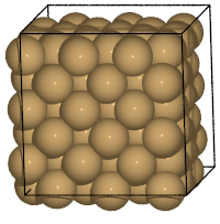
A visualization of the results is shown below.
Here, the read method has been set to index="::100" to visualize the results of interval thinning from the Trajectory file. Although Cu retains its solid structure and is not moving significantly, we can see that there is a change in the cell size due to the vibrational movement.
[2]:
from ase.io import Trajectory, read
from pfcc_extras.visualize.povray import traj_to_apng
from IPython.display import Image


traj = read("./output/ch6/fcc-Cu_3x3x3_NPT_EMT_0900K.traj", index="::100")
traj_to_apng(traj, f"output/ch6/Fig6-3_fcc-Cu_3x3x3_NPT_EMT_0900K.png", rotation="10x,-10y,0z", clean=True, n_jobs=16)

Image(url="output/ch6/Fig6-3_fcc-Cu_3x3x3_NPT_EMT_0900K.png")
[Parallel(n_jobs=16)]: Using backend ThreadingBackend with 16 concurrent workers.
[Parallel(n_jobs=16)]: Done  12 out of  21 | elapsed:    5.8s remaining:    4.4s
[Parallel(n_jobs=16)]: Done  21 out of  21 | elapsed:    7.2s finished
[2]:
[3]:
from ase.io import Trajectory, read
from pfcc_extras.visualize.view import view_ngl


traj = read("./output/ch6/fcc-Cu_3x3x3_NPT_EMT_0900K.traj", index="::100")
view_ngl(traj, replace_structure=True)
[3]:
The time constant \(\tau_t\) of the heat bath is 20 fs and the barostat parameter, pfactor, is 2e6 GPa\(\cdot\)fs\(^2\). Let’s check how the cell volume changes with time during a 20 ps NPT-MD simulation at 300 K to achieve thermal equilibrium under the above calculation conditions. You can analyze the traj file, which is the result of MD simulation at a specific temperature, with the following code.
[4]:
import matplotlib.pyplot as plt
from pathlib import Path
from ase.io import read,Trajectory

time_step = 0.01  # Time step size in ps between each snapshots recorded in traj
traj = Trajectory("./output/ch6/fcc-Cu_3x3x3_NPT_EMT_0300K.traj")

time = [ i*time_step for i in range(len(traj)) ]
volume = [ atoms.get_volume() for atoms in traj ]

# Create graph
fig = plt.figure(figsize=(8,3))
ax = fig.add_subplot(1, 1, 1)
ax.set_xlabel('time (ps)')  # x axis label
ax.set_ylabel('Cell volume (Å^3)')  # y axis label
ax.plot(time,volume, alpha=0.5)
ax.set_ylim([1100,1400])
#plt.savefig("filename.png")  # Set filename to be saved
plt.show()
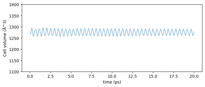
The time evolution of the cell volume for a 20 ps NPT-MD simulation at 300 K to achieve thermal equilibrium under these calculation conditions is shown below.
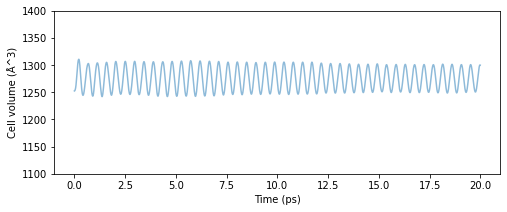
Fig.6-3a. Time evolution of cell volume. (fcc-Cu_3x3x3, @300 K and 1 bar)
It is shown that the cell volume oscillates within a range of about 4% with the NPT ensemble. Since we are dealing with cubic crystals, we can calculate the lattice constant of the crystal from the geometric mean of this volume, and by plotting the average normalized lattice constant at each temperature from 200 K to 1000 K, we obtain the following results. (Since we want to calculate the lattice constant after equilibrium is reached, we use only the second half of the Trajectory in the
np.mean(vol[int(len(vol)/2):])**(1/3) part to calculate the lattice constant from the volume.)
[5]:
import matplotlib.pyplot as plt
import numpy as np
from pathlib import Path
from ase.io import read,Trajectory

time_step = 10.0  # Time step size between each snapshots recorded in traj
paths = Path("./output/ch6/").glob(f"**/fcc-Cu_3x3x3_NPT_{calc_type}_*K.traj")
path_list = sorted([ p for p in paths ])

# Temperature list extracted from the filename
temperature = [ float(p.stem.split("_")[-1].replace("K","")) for p in path_list ]
print("temperature = ",temperature)

# Compute lattice parameter
lat_a = []
for path in path_list:
    print(f"path = {path}")
    traj = Trajectory(path)
    vol = [ atoms.get_volume() for atoms in traj ]
    lat_a.append(np.mean(vol[int(len(vol)/2):])**(1/3))

print("lat_a = ",lat_a)

# Normalize relative to the value at 300 K
norm_lat_a = lat_a/lat_a[1]
print("norm_lat_a = ",norm_lat_a)

# Plot
fig = plt.figure(figsize=(4,4))
ax = fig.add_subplot(1, 1, 1)
ax.set_xlabel('Temperature (K)')  # x axis label
ax.set_ylabel('Normalized lattice parameter')  # y axis label
ax.scatter(temperature[:len(norm_lat_a)],norm_lat_a, alpha=0.5,label=calc_type.lower())
ax.legend(loc="upper left")
temperature =  [200.0, 300.0, 400.0, 500.0, 600.0, 700.0, 800.0, 900.0, 1000.0]
path = output/ch6/fcc-Cu_3x3x3_NPT_EMT_0200K.traj
path = output/ch6/fcc-Cu_3x3x3_NPT_EMT_0300K.traj
path = output/ch6/fcc-Cu_3x3x3_NPT_EMT_0400K.traj
path = output/ch6/fcc-Cu_3x3x3_NPT_EMT_0500K.traj
path = output/ch6/fcc-Cu_3x3x3_NPT_EMT_0600K.traj
path = output/ch6/fcc-Cu_3x3x3_NPT_EMT_0700K.traj
path = output/ch6/fcc-Cu_3x3x3_NPT_EMT_0800K.traj
path = output/ch6/fcc-Cu_3x3x3_NPT_EMT_0900K.traj
path = output/ch6/fcc-Cu_3x3x3_NPT_EMT_1000K.traj
lat_a =  [10.821187657763522, 10.84284171781325, 10.866195382765163, 10.88834101681545, 10.91184951417741, 10.937661285868403, 10.958914931081702, 10.988423059467703, 11.016341565694251]
norm_lat_a =  [0.99800292 1.         1.00215383 1.00419625 1.00636436 1.0087449
 1.01070505 1.01342649 1.01600133]
[5]:
<matplotlib.legend.Legend at 0x7f2643b7a210>
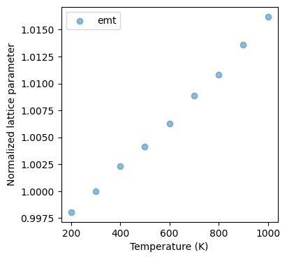
The following plot is obtained by running the above code.
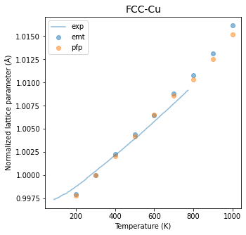
Fig.6-3b. Normalized lattice parameter as a function of temperature.
Experimental data is taken from Reference [4].
The results are further compared with the PFP calculations and, with the experimental data for reference. There is very good agreement for both the EMT and PFP data, while the PFP data appears to be closer to the experimental data with a small margin.
The coefficient of linear thermal expansion (CTE, \(\alpha\)) is calculated from the temperature dependence of the normalized lattice parameter using the following equation
where \(\alpha\) is the coefficient of linear thermal expansion and \(a(T)\) and \(a_{RT}\) are the lattice constants at temperature \(T\) and room temperature. The following is a summary of ASAP3-EMT, PFP, and experimental values [4].
\(\alpha\) ( \(10^{-5}\) /K) |
|
|---|---|
emt |
2.23 |
pfp |
2.13 |
exp |
1.74 |
Considering the calculation error, both calculation results are in reasonable agreement with the experimental values.
The coefficient of thermal expansion can be calculated by using MD simulations of the NPT ensemble in this way.
You may be thinking, “Can’t we reproduce thermal expansion of liquids and gases in the same way?” In principle, this is true, but at present there are only a limited number of models that can reproduce the thermal expansion of liquids and gases. There may be models that are specialized for specific liquids and gases in the classical force field, but when using first-principles calculations, the accuracy of intermolecular interactions in liquids and gases, which are much smaller than those in solids, is critical, and quantum chemical calculations with such accuracy are currently very difficult to perform. In particular, a large amount of computational data is required to create NNPs, and it is currently not very realistic to perform a large number of high-precision quantum chemical calculations. Therefore, the development of models with high accuracy in this area is expected in the future.
[Advanced] Parrinello-Rahman barostat parameter dependency
When performing MD simulations in the NPT ensemble, a parameter called pfactor needs to be chosen. It was explained that the appropriate value range is around 10\(^6\) GPa\(\cdot\)fs\(^2\) to 10\(^7\) GPa\(\cdot\)fs\(^2\). For your reference, the results when changing the value of pfactor are shown below. The calculation targets are the same fcc-Cu 3x3x3 unit cells as above, and the temperature is 300 K.
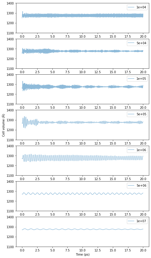
Fig.6-3c. Time evolution of cell volume as a function of pfactor.
When pfactor is small, the cell volume is oscillating at high speeds which is not desirable, and some regions have a mixture of high and low frequency oscillations making the system unstable. As pfactor increases, the period of oscillation gradually increases, and the large volume changes at the beginning of the calculation are hardly noticeable. Although there is no clear cut indicator of which value of pfactor is correct, the median value seems to be as stable as ever, although
small oscillations can be observed for values of 10\(^6\) Ga\(\cdot\)fsec\(^2\) or higher. Similarly, there is no well-defined reference for the upper limit, and since the larger the pfactor, the longer the oscillation period becomes and the more difficult it is to handle. A range between 10\(^6\) and 10\(^7\) seems appropriate for the above example.
[Advanced] Berendsen barostat parameter dependency
Here, we explain the calculation method using Berendsen barostat. The time evolution of pressure is calculated according to the following equation. (For details of the derivation, see reference [5]).
It is clear from the above equation that the Berendsen pressure control method exponentially increases the pressure at each time in the system closer to the external pressure \(\mathbf{P}_o\). Its speed is controlled by the time constant \(\tau_P\).
At each MD step, the coordinates and cell vectors of each atom are scaled by a factor expressed by the following equation
Just as \(\tau_T\) was a time constant when controlling a heat bath, an appropriate time constant \({\tau_P}\) must be set for the pressure control method. Let’s look at an actual calculation example.
Using the NPTBerendsen class, the object defining the dynamics is written in the following form
[6]:
from ase.md.nptberendsen import NPTBerendsen

dyn = NPTBerendsen(
    atoms,
    time_step*units.fs,
    temperature_K = temperature,
    pressure_au = 1.0 * units.bar,
    taut = 5.0 * units.fs,
    taup = 500.0 * units.fs,
    compressibility_au = 5e-7 / units.bar,
    logfile = log_filename,
    trajectory = traj_filename,
    loginterval=num_interval
)
Inhomogeneous_NPTBerendsen, which handles anisotropic pressure control, can be used with the same setting. (Simply relacing the class name from NPTBerendsen to Inhomogeneous_NPTBerendsen should work.) One difference between the two classes is that Inhomogeneous_NPTBerendsen accept mask argument can be set, i.e. setting mask=(1, 1, 1) allows the cell paramters a, b, and c can vary independently. If the element of this tuple is set to 0, the cell is fixed in that direction.
In addition to the calculation conditions such as temperature and pressure, it is necessary to set parameters called barostat time constant (taup, \(\tau_P\)) and compression ratio (compressibility, \(\beta_T\)). The dependence of the time variation of the cell volume on each of these values will be checked using the example of fcc-Cu at 300 K. We will start with \(\tau_P\).
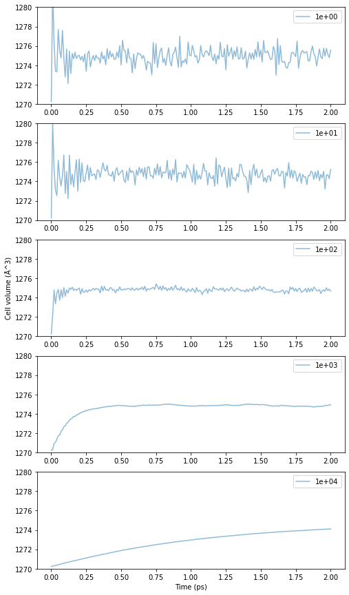
Fig.6-3d. Time evolution of cell volume as a function of \(\tau_P\).
The smaller the time constant, the more unstable and violent the period of oscillation is. On the other hand, if the time constant is too large, the change is too gradual and it takes time to reach equilibrium. This is the same concept as the time constant of the heat bath method. For a system mechanically similar to fcc-Cu, the appropriate value for \(\tau_P\) is around 10\(^2\) fs to 10\(^3\) fs due to the stability and convergence of the volume change.
Next is the dependence on \(\beta_T\). The results are as follows.
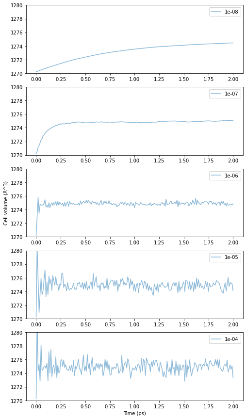
Fig.6-3e. Time evolution of cell volume as a function of \(\beta_T\).
The smaller \(\beta_T\) is, the slower the convergence is, and the higher the value, the more unstable it becomes. From the trend of the graph, 10\(^{-7}\) to 10\(^{-6}\)fs seems to be a good range for \(\beta_T\).
There is no strict guideline for choosing the values of \(\tau_P\) and \(\beta_T\). But it is better to have the sense of the trend when these values are changed by an order of magnitude.
Finally, it should be noted that these values are only applicable to dense metallic materials such as fcc-Cu. If one wants to treat a completely different kind of materials (e.g., polymers, liquids, gases, etc.) with NPT ensemble, the appropriate range of values should be studied in advance. In general, it is recommended that great care be taken when working with new material systems, as omitting this preliminary study may lead to unintended results and extra time.
Reference
[1] M.E. Tuckerman, “Statistical mechanics: Theory and molecular simulation”, Oxford University Press (2010) ISBN 978-0-19-852526-4. https://global.oup.com/academic/product/statistical-mechanics-9780198525264?q=Statistical%20mechanics:%20Theory%20and%20molecular%20simulation&cc=gb&lang=en#
[2] Melchionna S. (2000) “Constrained systems and statistical distribution”, Physical Review E 61 (6) 6165 https://journals.aps.org/pre/abstract/10.1103/PhysRevE.61.6165
[3] S. Melchionna, G. Ciccotti, B.L. Holian, “Hoover NPT dynamics for systems varying in shape and size”, Molecular Physics, (1993) 78 (3) 533 https://doi.org/10.1080/00268979300100371
[4] F.C. Nix, D. MacNair, “NIST:The Thermal Expansion of Pure Metals: Copper, Gold, Aluminum, Nickel, and Iron” https://materialsdata.nist.gov/handle/11256/32
[5] H. J. C. Berendsen, J. P. M. Postma, W. F. van Gunsteren, A. DiNola, and J. R. Haak, “Molecular dynamics with coupling to an external bath”, J. Chem. Phys. (1984) 81 3684 https://aip.scitation.org/doi/10.1063/1.448118