ASE Calculator
In the previous section, we learned the basics about ASE Atoms and how to generate structures.
In this section, we will learn how to handle Calculator, which is necessary for physical simulations.
Energy
The total energy \(E\) of the system is expressed in terms of the kinetic energy \(K\) and the potential energy \(V\).
Of these, the kinetic energy \(K\) of atoms can be calculated as follows, from classical mechanics.
where \(m_i, \mathbf{v}_i, \mathbf{p}_i\) are the mass, velocity and momentum (\(\mathbf{p}=m\mathbf{v}\)) of each atom, respectively.
Those in bold represent vectors, where the velocity \(\mathbf{v}\) and momentum \(\mathbf{p}\) have three components in xyz coordinates.
On the other hand, the potential energy \(V\) is not easy to obtain exactly because it requires solving equations derived from quantum mechanics (e.g., Schrödinger equation, see column). There are various methods for determining potential energy, ranging from classical force fields, which is fast but limited in its applicability, to quantum chemical calculations such as the density functional theory (DFT), which takes longer but is more accurate (The differences between these methods are discussed below).
So why do we want to know about energy in the first place? In another word, what can we learn from energy?
First, we can know the stable structure of a substance, which is not self-evident in nature (as explained in chapter 2). By looking at the low and high energies, we can analyze whether the structure is realized in nature or not.
Second, we can learn how each atom moves. This will be explained in the next section.
Force
In classical mechanics, Newton’s equations of motion are expressed as follows
This equation represents that given a force \(\mathbf{F}\), we know the acceleration \(\mathbf{a}\) applied to the system.
The position \(\mathbf{r}\), velocity \(\mathbf{v}\), and acceleration \(\mathbf{a}\) of each atom are related as follows.
Therefore, when we know the force, we know the acceleration (= how the velocity changes), and as a result, we know how the position evolves over time. MD (Molecular Dynamics), which actually deals with time evolution in this way, is covered in chapter 6.
The forces can be expressed as the derivative of the potential energy with resprect to positions.
In summary, the force \(\mathbf{F}\), required to know the time evolution \(\mathbf{r}(t)\) of the system, can be calculated if the potential energy \(V\mathbf(r)\) is known.
[Note] For the sake of simplicity, this tutorial has been explained using only knowledge of classical mechanics. For those who have studied analytical mechanics, the governing equations are defined by the Hamiltonian. Knowing the Hamiltonian (the function related to the energy mentioned above) allows us to describe the time evolution of the system.
Calculator class
We have explained that once the potential energy \(V(\mathbf{r})\) is determined, we know the governing equations of system, that is, how the atoms move in this world.
In ASE, the Calculator class is in charge of calculating the potential energy, and the calculation method can be switched by switching Calculator.
Let’s look at one example. The following is a calculation of each energy of H2 using the PFP calcultor provided by Matlantis.
The detailed usage is described later, but you can calculate each energy by setting Calculator for atoms.calc. In this example, we use below methods to calculate each energy.
Total energy \(E\):
atoms.get_total_energy()Potential energy \(V\):
atoms.get_potential_energy()Kinetic energy \(K\):
atoms.get_kinetic_energy()
[1]:
from ase import Atoms

import pfp_api_client
from pfp_api_client.pfp.calculators.ase_calculator import ASECalculator
from pfp_api_client.pfp.estimator import Estimator, EstimatorCalcMode


# print(f"pfp_api_client: {pfp_api_client.__version__}")

estimator = Estimator(calc_mode=EstimatorCalcMode.PBE, model_version="v8.0.0")
calculator = ASECalculator(estimator)
[2]:
atoms = Atoms("H2", [[0, 0, 0], [1.0, 0, 0]])
atoms.set_momenta([[0.1, 0, 0], [-0.1, 0, 0]])
atoms.calc = calculator

E_tot = atoms.get_total_energy()
E_pot = atoms.get_potential_energy()
E_kin = atoms.get_kinetic_energy()

print(f"Total Energy     : {E_tot:f} eV")
print(f"Kinetic Energy   : {E_kin:f} eV")
print(f"Potential Energy : {E_pot:f} eV")
Total Energy     : -3.855425 eV
Kinetic Energy   : 0.009921 eV
Potential Energy : -3.865346 eV
Atoms initially have an initial velocity of 0 and kinetic energy of 0, so an appropriate initial velocity is set using the set_momenta function.
You can see that $ E = K + V $.
The Calculator is necessary to calculate the total energy \(E\) and potential energy \(V\), and without the atoms.calc = calculator setting, the calculation cannot be performed and an error will be raised.
Calculator type
ASE supports a variety of calculators, from classical force fields to calculators using quantum chamical calculations. Some examples are listed below. Many other calculators are supported in addition to those listed here. Please check Supported calculators for details.
Category | Calculator | ASE embedded | Description |
|---|---|---|---|
Classical force field | lj | ✓ | Lennard-Jones potential |
morse | ✓ | Morse potential | |
emt | ✓ | Effective Medium Theory calculator | |
lammps | Classical molecular dynamics code | ||
Quantum chemical calculations | gaussian | Gaussian based electronic structure code | |
vasp | Plane-wave PAW code | ||
espresso | Plane-wave pseudopotential code | ||
NNP (Neural Network Potential) | PFP | Potential provided by Matlantis |
Calculators with ✓ in the “ASE embedded” column above can be used simply by installing ASE, other calculators require to install external program.
Calculators that perform quantum chemical calculations theoretically calculate potentials by solving the Schrödinger equation derived from quantum mechanics under a certain approximation (see also the column below). Special software is required and some calculations are time-consuming. It is used when you want to perform more accurate calculations.
https://en.wikipedia.org/wiki/Lennard-Jones_potential
The calculators belonging to classical force fields are methods that calculate potentials using manually created (empirical) function formulas, e.g., Lennard-Jones potential, Morse potential. The calculation speed is fast, but each method can handle different structures and physical phenomena. You need validation to check if the potential works for your interest.
The NNP type is intended to perform highly accurate potential prediction in a fast computation time by preparing many data computed in advance using quantum chemical calculations, and by supervised learning of the relationship between input structures and their potential energies. For more information on NNP, please refer to the following slides as well.
PFP:材料探索のための汎用Neural Network Potential - 2021/10/4 QCMSR + DLAP共催 (currently Japanese only)
ASE embedded calculator
Here we use EMT calculator as an example.
[3]:
from ase.build import bulk
from ase.calculators.emt import EMT


calculator_emt = EMT()

atoms = bulk("Cu")
atoms.calc = calculator_emt

E_pot_emt = atoms.get_potential_energy()
print(f"Potential energy {E_pot_emt:.5f} eV")
Potential energy -0.00568 eV
The calculator can be switched to perform atomistic simulations in this way.
If the exact potential energy \(V(\mathbf{r})\) could be calculated quickly, there would be no need to switch calculators and the simulation could always be run using that, but in reality the exact potential energy cannot be calculated, and there is a tradeoff between accuracy and speed. Therefore, the choice must be made by the user of the atomistic simulation to suit the application.
PFP
The PFP provided by Matlantis is characterized by universality and high speed. It can be used to perform fast calculations for systems with a variety of structures in combinations of 55 elements.
PFP calculator is usually used in this tutorial throughout.
[4]:
import pfp_api_client
from pfp_api_client.pfp.calculators.ase_calculator import ASECalculator
from pfp_api_client.pfp.estimator import Estimator, EstimatorCalcMode

estimator = Estimator(calc_mode=EstimatorCalcMode.PBE, model_version="v8.0.0")
calculator = ASECalculator(estimator)

atoms.calc = calculator

E_pot_emt = atoms.get_potential_energy()
print(f"Potential energy {E_pot_emt:.5f} eV")
Potential energy -3.50745 eV
The absolute values of the energies are very different between EMT and PFP above, but their absolute values are arbitrary to shift when defining the energy of the system.
Note that the difference between the energies of two different systems consisting of the same number of atoms is meaningful, but the absolute values of each are not so meaningful.
Relation between Atoms and Calculator
In the ASE library, the atomic structure is represented by the Atoms class, and each basic physical property value (energy, force, stress, charge, etc.) for the Atoms can be calculated by setting Calculator to it. Calculator is set directly to atoms.calc.
Relation between Atoms and Calculator
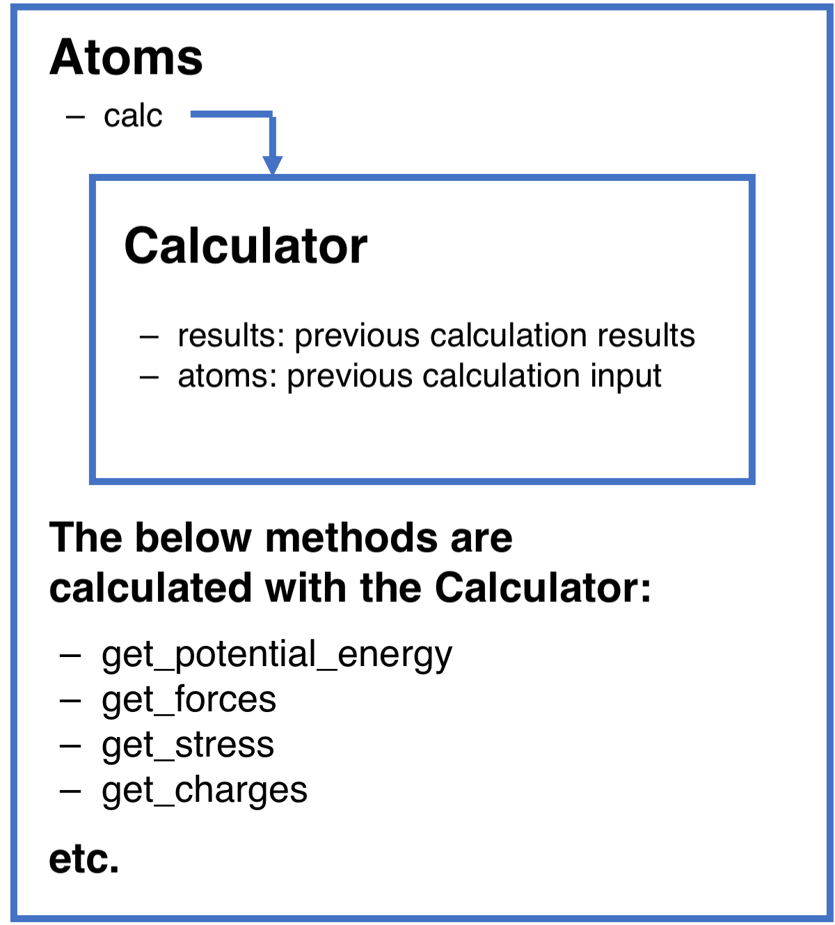
The basic physical properties that can be calculated via Calculator and their calculation methods are as follows.
Potential energy:
get_potential_energyForce:
get_forcesStress:
get_stressCharge:
get_chargesMagnetic moment:
get_magnetic_momentDipole moment:
get_dipole_moment
[5]:
calculator = ASECalculator(Estimator())

atoms = bulk("Pt") * (2, 2, 1)
atoms.calc = calculator

E_pot = atoms.get_potential_energy()
charges = atoms.get_charges()
forces = atoms.get_forces()
stress = atoms.get_stress()

print(f"E_pot {E_pot:.2} eV")
print(f"charges {charges} C")
print(f"forces {forces} eV/A")
print(f"stress {stress} eV/A^2")
E_pot -2.2e+01 eV
charges [ 9.43063085e-08 -1.33015320e-07  3.13127657e-08  7.39626715e-09] C
forces [[-3.91123683e-07 -1.43381488e-06 -1.13995344e-07]
 [ 1.25751198e-07  7.27608341e-07 -4.82172099e-07]
 [ 3.08472670e-07  6.67509722e-07  6.51636428e-07]
 [-4.31001849e-08  3.86968210e-08 -5.54689846e-08]] eV/A
stress [-6.11363515e-02 -6.11362953e-02 -6.11362604e-02 -4.56216412e-08
 -1.29756214e-08  2.64759676e-08] eV/A^2
PFP does not support the calculation of magnetic moments or dipole moments. (The magnetic moment is for electronic states and is not used in atomistic simulation, which is the scope of this tutorial.)
[6]:
# Some Calculator supports this, but PFP calculator raises error.

# magmom = atoms.get_magnetic_moment()
# dipole = atoms.get_dipole_moment()
The following [columns] contain advanced content, and can be skipped as you read through the tutorial.
[Column] Calcultor’s cache mechanism
Calculator stores the input atomic structure of the previous calculation in calculator.atoms and the result of the previous calculation in calculator.results. If you call the get_XXX method for the same atomic structure as before, it will skip the re-calculation.
[7]:
atoms.calc = calculator
calculator.reset()
[8]:
%time Epot = atoms.get_potential_energy()
%time Epot = atoms.get_potential_energy()
CPU times: user 4.56 ms, sys: 74 μs, total: 4.63 ms
Wall time: 54.7 ms
CPU times: user 394 μs, sys: 57 μs, total: 451 μs
Wall time: 376 μs
Comparing the wall time in the above example, we can see that the first run takes time on the order of milliseconds and calculations are performed, but the second run skips the calculations, so the energy is obtained in less than a millisecond.
calculator.reset() can be used to explicitly clear the cache of calculation results and recalculate them. In the following example, you can see that the second calculation still takes milliseconds of calculation time.
[9]:
calculator.reset()

print("----- 1st calc -----")
%time Epot = atoms.get_potential_energy()

print(f"After 1st calc   : {calculator.results}")
calculator.reset()
print(f"After reset      : {calculator.results}")

print("----- 2nd calc -----")
%time Epot = atoms.get_potential_energy()
print(f"After 2nd calc   : {calculator.results}")
----- 1st calc -----
CPU times: user 787 μs, sys: 3.59 ms, total: 4.37 ms
Wall time: 43.1 ms
After 1st calc   : {'energy': -21.83327454244104, 'forces': array([[ 5.79606318e-07,  1.16643336e-08, -7.64247158e-07],
       [ 4.26722455e-07, -6.91453473e-07,  2.31298103e-07],
       [-1.04722843e-06,  1.10711275e-06,  9.41913682e-07],
       [ 4.08996548e-08, -4.27323608e-07, -4.08964628e-07]]), 'charges': array([-2.03779976e-07,  2.57427558e-07, -2.57081929e-08, -2.79393912e-08]), 'calc_stats': {'elapsed_usec_preprocess': 2670, 'elapsed_usec': 35434, 'elapsed_usec_infer': 14317, 'n_atoms_plus_ghost_atoms': 648, 'n_neighbors_after_screening': 181, 'n_neighbors': 400}, 'free_energy': -21.83327454244104, 'stress': array([-6.11363107e-02, -6.11362962e-02, -6.11363219e-02, -2.04317220e-09,
        2.01130126e-08,  2.54945406e-08])}
After reset      : {}
----- 2nd calc -----
CPU times: user 1.88 ms, sys: 279 μs, total: 2.16 ms
Wall time: 65.8 ms
After 2nd calc   : {'energy': -21.83327428830643, 'forces': array([[-2.58579924e-07, -9.56917804e-07, -3.05839054e-07],
       [ 1.61156848e-06, -6.46716022e-07,  8.28612038e-07],
       [-6.34963105e-07,  1.14477575e-06,  2.37882247e-08],
       [-7.18025455e-07,  4.58858077e-07, -5.46561208e-07]]), 'charges': array([ 1.54533186e-08, -1.24843197e-07,  3.70590563e-08,  7.23307920e-08]), 'calc_stats': {'elapsed_usec_preprocess': 2707, 'elapsed_usec': 50686, 'elapsed_usec_infer': 11449, 'n_atoms_plus_ghost_atoms': 648, 'n_neighbors_after_screening': 874, 'n_neighbors': 400}, 'free_energy': -21.83327428830643, 'stress': array([-6.11357170e-02, -6.11356858e-02, -6.11355888e-02,  2.65571912e-08,
       -3.69590628e-08,  3.96031769e-08])}
Note that if the atomic structure changes even slightly, the result of calculator.result is discarded and a new calculation is performed.
In the following example, atoms.get_potential_energy is called again after changing the interatomic distance of the hydrogen molecule, and in this case, Calculator detects the change in the input atomic structure and performs a new calculation. You can see that both calculations actually take a wall time on the order of milliseconds.
[10]:
atoms = Atoms(["H", "H"], positions=[[0, 0, 0], [0, 0, 0.8]])

atoms.calc = calculator
%time E_pot1 = atoms.get_potential_energy()
# --- calculator.atoms stores the previously calculated atoms
# print(calculator.atoms.positions)

# Change atomic distance to 2A
atoms.positions[1, 2] = 2.0
# --- The preveously calculated `calculator.atoms` and current calculate target `atoms` are
# different, so calculation is executed.
%time E_pot2 = atoms.get_potential_energy()
# print(calculator.atoms.positions)

print(f"E_pot1 {E_pot1:.2f} eV")
print(f"E_pot2 {E_pot2:.2f} eV")
CPU times: user 4.62 ms, sys: 0 ns, total: 4.62 ms
Wall time: 67.7 ms
CPU times: user 3 ms, sys: 204 μs, total: 3.21 ms
Wall time: 80.1 ms
E_pot1 -4.49 eV
E_pot2 -0.13 eV
[Column] PFP Calculator behavior
※This section is a description of Matlantis-specific behavior.
It describes the behavior of the ASECalculator provided by the pfp-api-client library.
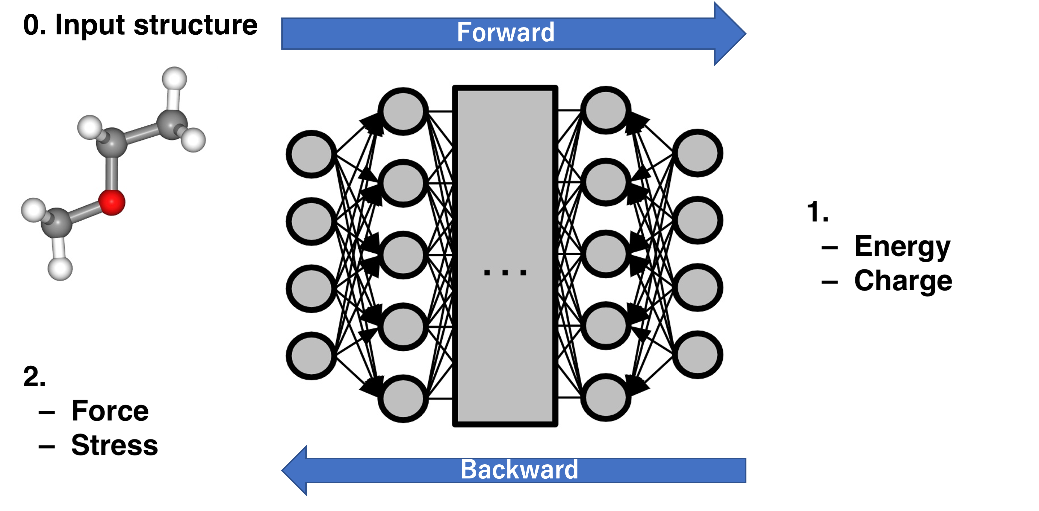
In PFP, potential_energy and charge are calculated by NNP’s forward, and forces and stress are calculated by NNP’s backward.
[Column] Potential energy obtained by quantum chemical calculations
In the explanation of total energy at the top of this tutorial, the formula for kinetic energy was given, but there was no formula for potential energy, only explained that it is calculated by Calculator. How is this potential energy expressed theoretically?
If you want to simulate phenomena occurring at the microscopic atomic scale, you will need the theory of quantum mechanics in order to determine the energies, etc., taking into account the electronic states of the system. In the case of the steady state, the Schrödinger equation given below gives the wave function \(\Phi\) and total energy \(E\) for the entire system.
Based on non-relativistic theory, the Hamiltonian \(\mathcal{H}\) for a system consisting of M nuclei and N electrons can be written as follows by atomic unit system.
\(M_A\): Mass of nucleus \(A\).
\(R_{AB}\): Distance between nucleus \(A\) and nucleus \(B\).
\(r_{Ai}\): Distance between nucleus \(A\) and electron \(i\).
\(r_{ij}\): Distance between electron \(i\) and electron \(j\).
\(Z_A\): Atomic number of nucleus \(A\) = number of protons.
and all electrons have charge -1.
The first item corresponds to the kinetic energy of electrons, the second to the kinetic energy of nuclei, the third to the electrostatic interaction energy between electrons and nuclei, the fourth to the electrostatic interaction energy between electrons, and the fifth to the electrostatic interaction energy between nuclei.
Since it is difficult to solve this as is, and a Born-Oppenheimer approximation is often used. Electrons move faster than nuclei because they are much lighter than nuclei. Therefore, the idea is to find the steady state of the electron at that time, assuming that the atom is perfectly stationary.
Then the Schrödinger equation for N electrons is
and
The total energy of the nucleus at stationary is written by
This corresponds to the potential energy.
If we can solve this, we should be able to obtain the potential energy from the fundamental laws of quantum mechanics alone, without introducing any parameters as in the classical force field. A calculation method based on quantum mechanics that does not depend on experimental values other than the fundamental physical constants is called first-principles calculation (ab initio calculation).
In reality, it is known that the Schrödinger equation (1) for this electron system cannot be solved analytically, and various approximations and assumptions are made by different methods. The Hartree-Fock method and DFT (density functional theory) are typical examples.
So, the potential energy \(V\) handled by ASE is a value that includes the electrostatic potential of electrons and nuclei plus the kinetic energy of electrons, and the kinetic energy \(K\) can be taken as the kinetic energy of nuclei only.
[Reference]
“MODERN QUANTUM CHEMISTRY Introduction to Advanced Electronic Structure Theory”, Attila Szabo and Neil S. Ostlund