Phonon

1. Introduction

1.1 What is phonon?

Essentially, a phonon is the vibration mode of atoms in the crystal. Before we go to the concepts, let’s look at what is a phonon from this website.

Animation visualization of phonon. Cite from http://henriquemiranda.github.io/phononwebsite/phonon.html.

Let’s open the website -> select Si in the left-upper materials column -> click any point in right figure, i.e. phonon dispersion. Then, you can see every atom (yellow ball) in the middle window shows periodic motion, and the collection movement of all atoms seems like a wave that travels from one end to another.

Such a vibration mode in the crystal is called lattice vibration. Lattice vibration usually deals with quantum effects and it is called “Phonon”. In this tutorial explanation, we don’t distinguish between the term lattice vibration and phonon. Please refer appendix & reference books for more detail.

The direction of wave propagation is usually represented by a vector \(\vec q\) (called wave vector). The most important problem in the phonon analysis is to know what kind of vibration modes are allowed for a given wave vector \(\vec q\), and the frequency of atomic vibration in those vibration modes.

Phonon is a kind of quasiparticle. It has energy (\(E\)) and momentum (\(\mathbf{p}\)). The phonon in a solid is directly related to its thermal and acoustic properties. For example, the excitation of a phonon causes the increase of internal energy (\(U\)); the transportation of the phonon causes the conduction of sound and heat. As a consequence, phonon analysis has been a very important simulation tool to obtain the properties of solids.

1.2 How to calculate the phonon frequency?

Similar to the vibration analysis (section 4-1), the phonon is also calculated with the harmonic approximation. However, the atom interacts with those in the neighboring unit cell in the crystal. By considering the periodical boundary condition, the potential energy of a small distorted crystal structure can be expressed as:

\[V(\mathbf{r}) \approx V(\mathbf{r_0}) +　\frac{1}{2} \sum_{ij} \frac{\partial^2 V(\mathbf{r_0})}{\partial r_i^a \partial r_j^b} \Delta \mathbf{r}_i^a \Delta \mathbf{r}_j^b\]

where, \(r_i^a\) indicates the coordination of the \(i\)-th atom at the \(a\)-th supercell. The force constant (explained in section 4-1) of a crystal should be a \(3NM \times 3NM\) matrix, where \(N\) is the number of atoms per unit cell and \(M\) is the number of the unit cell to be considered. The force constant can be a very large matrix.

We assume that the atomic displacement from its equilibrium position \(u\) in a vibration mode in the crystal should have the following form (plane-wave-like function)

\[u(\vec R, t) = A e^{ \vec{q} \vec{R} -i\omega_{m} t}\]

Then, the large force constant matrix can be converted into a \(3N \times 3N\) dynamical matrix by discrete Fourier transform in real space. The dynamical matrix depends on the wave vector \(\vec q\). The eigenvalue and eigenvector of the dynamical matrix are the vibration frequencies and vibration modes of the phonon. For a detailed explanation of the phonon calculation formula, please refer to the appendix.

In the next section, we show how to calculate the phonon properties using the matlantis-features package. Some important concepts of phonon are introduced at the same time.

2. Example: phonon calculation of Si

2.1 Material preparation

Here, we use crystal silicon as an example to run the phonon calculation. As the first step, we should relax the crystal structure. Usually, we use the primitive cell of the crystal to calculate phonon dispersion since it contains the least number of atoms.

import numpy as np
np.set_printoptions(precision=3)

from ase.build import bulk
from ase.optimize import BFGS
from ase.constraints import ExpCellFilter

import pfp_api_client
from pfp_api_client.pfp.calculators.ase_calculator import ASECalculator
from pfp_api_client.pfp.estimator import Estimator, EstimatorCalcMode

estimator = Estimator(calc_mode=EstimatorCalcMode.CRYSTAL, model_version="v3.0.0")
calculator = ASECalculator(estimator)
atoms = bulk("Si")
atoms.calc = calculator

exp = ExpCellFilter(atoms)
BFGS(exp).run(fmax=0.01)

      Step     Time          Energy          fmax
BFGS:    0 14:31:50       -9.108033        0.496677
BFGS:    1 14:31:50       -9.113258        0.001942

/tmp/ipykernel_17542/260060846.py:17: FutureWarning: Import ExpCellFilter from ase.filters
  exp = ExpCellFilter(atoms)

True

2.2 Calculation of force constant matrix

Same with the vibration analysis, the force constant is necessary for calculating the vibration frequencies of phonons. Here, we obtain the force constant of the crystal using the ForceConstantFeature.

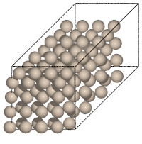
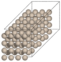
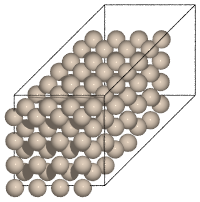
The primitive cell of crystal Si contains only 2 atoms. We should repeat the unit cell many times to obtain an accurate result. It is because the force constant element \(\frac{\partial^2 V(\mathbf{r_0})}{\partial r_i^a \partial r_j^b}\) will decay with the distance between atoms \(i\) of unit cell \(a\) and the atoms \(j\) of unit cell \(b\). Only if the supercell is large enough, all non-negligible elements of the force constant matrix can be included. In this example, we expand the crystal Si structure by 10x10x10 time.

The ForceConstantFeature in matlantis-features is used to compute the force constant of crystal silicon.

from matlantis_features.features.phonon import ForceConstantFeature

fc = ForceConstantFeature(
    supercell = (10,10,10),
    delta = 0.1,
)
force_constant = fc(atoms)
print(force_constant.force_constant.shape)

/home/jovyan/.py39/lib/python3.9/site-packages/matlantis_features/features/phonon/force_constant.py:95: UserWarning: Model version is not specified, default 'v7.0.0' will be used.Please specify it by providing an estimator_fn or setting the 'MATLANTIS_PFP_MODEL_VERSION' environment variable.
  self.check_estimator_fn(estimator_fn)
/home/jovyan/.py39/lib/python3.9/site-packages/matlantis_features/features/phonon/force_constant.py:95: UserWarning: Calculation mode is not specified, default 'EstimatorCalcMode.CRYSTAL_U0' will be used.Please specify it by providing an estimator_fn or setting the 'MATLANTIS_PFP_CALC_MODE' environment variable.
  self.check_estimator_fn(estimator_fn)

(1000, 6, 6)

The calculation result, i.e. force constant \(C\), is a 1000x6x6 tensor.

print(force_constant.force_constant[1])

[[-0.218 -0.193 -0.092 -0.01   0.015  0.056]
 [-0.193 -0.218 -0.092  0.015 -0.01   0.056]
 [ 0.092  0.092  0.433  0.056  0.056 -0.096]
 [-3.081 -2.114  2.114 -0.218 -0.193  0.092]
 [-2.114 -3.081  2.114 -0.193 -0.218  0.092]
 [ 2.114  2.114 -3.081 -0.092 -0.092  0.433]]

The force_constant.force_constant[1] is a 6x6 tensor. It is the force constant between the first and second unit cell \(C^{1,2}\), i.e. $:nbsphinx-math:frac{partial^2 V(mathbf{r_0})}{partial r_i^1 partial r_j^2} $. Same as the vibration analysis, the element of \(C^{1,2}\) is approximated with the finite differences method.

\[C^{1,2}[i,j]=\frac{\partial^2 V(\mathbf{r_0})}{\partial r_i^1 \partial r_j^2} \approx \frac{F(\mathbf{r_0} + \Delta r_i^1)_j^2 - F(\mathbf{r_0})_j^2}{|\Delta{r_i^1}|}\]

Since we used 10x10x10 unit cells, we should have 1000x1000 such a 6x6 matrix. However, the crystal has translational invariance, which makes the \(C^{a,b} = C^{0, b-a}\). Thus, we can represent the force constant with a 1000x6x6 tensor.

2.3 Calculation of dynamical matrix

Unlike the molecular vibration, in which the vibration frequency is obtained from diagonalization of force constant \(C\), the vibration frequency of the crystal is the eigenvalue of the dynamical matrix \(D_{\vec q}\), which is the discrete Fourier transform of the force constant in the real space. To obtain the dynamical matrix, we introduced another parameter, wave vector \(\vec q\).

Then, we use the PhononFreqency provided by matlantis-features to obtain the dynamical matrix of crystal silicon for the wave vector \(\vec q = [0.1, 0.0, 0.0]\).

from matlantis_features.features.phonon.utils import PhononFrequency

phonon_frequency = PhononFrequency(
    force_constant.force_constant, force_constant.supercell, force_constant.unit_cell_atoms
)
dynamic_matrix = phonon_frequency._dynamic_matrix_q(np.array([0.1, 0.0, 0.0])).real
print("Dynamical matrix of q=[0.1, 0.0, 0.0]:")
print(dynamic_matrix)

Dynamical matrix of q=[0.1, 0.0, 0.0]:
[[ 0.443 -0.004 -0.004 -0.419 -0.011 -0.011]
 [-0.004  0.443  0.004 -0.011 -0.418  0.011]
 [-0.004  0.004  0.443 -0.011  0.011 -0.418]
 [-0.419 -0.011 -0.011  0.443 -0.004 -0.004]
 [-0.011 -0.418  0.011 -0.004  0.443  0.004]
 [-0.011  0.011 -0.418 -0.004  0.004  0.443]]

The dynamical matrix is a symmetric 6x6 matrix. It is calculated from the force constant \(C\) with the following formula.

\[\tilde{D}_{\vec{q}}[k\alpha, k'\beta] = \frac{1}{\sqrt{M_k M_{k'}}} \tilde{C}(\vec{q})[k\alpha, k'\beta]\]

\[\tilde{C}_{\vec{q}}[k\alpha, k'\beta] = \sum_{b} {\left( \frac{\partial ^{2} E}{\partial{u_{k}^{a\alpha}} \partial{u_{k'}^{b\beta}}} \right) e^{i\vec{q}(\vec{R_b} - \vec{R_a})}} = \sum_{b} {C^{0,b}[k\alpha, k'\beta] e^{i\vec{q}(\vec{R_b} - \vec{R_a})}}\]

Then, we can diagonalize this matrix and obtain the eigenvalue and eigenvector. Same as molecular vibration, the eigenvalue is the vibration frequency of the phonon, and the eigenvector is related to the displacement of atoms in the phonon mode. Please see the appendix for the deduction of above equations.

So, let’s get the phonon frequency of crystal silicon at \(\vec q = [0.1, 0.0, 0.0]\).

frequency, eigenvector = phonon_frequency._frequency_mode_q(np.array([0.1, 0.0, 0.0]), return_mode=True)
for i in range(6):
    print(f"Band {i}")
    print(f"    Frequency: {frequency[i]:.3f} meV")
    print(f"    Eigenvector:")
    print(eigenvector[i].real)

Band 0
    Frequency: 6.116 meV
    Eigenvector:
[[-0.109 -0.049 -0.06 ]
 [-0.108 -0.049 -0.06 ]]
Band 1
    Frequency: 6.116 meV
    Eigenvector:
[[ 0.006  0.097 -0.091]
 [ 0.006  0.097 -0.091]]
Band 2
    Frequency: 11.568 meV
    Eigenvector:
[[ 0.073 -0.073 -0.073]
 [ 0.077 -0.077 -0.077]]
Band 3
    Frequency: 60.273 meV
    Eigenvector:
[[-0.072  0.073  0.073]
 [ 0.076 -0.078 -0.077]]
Band 4
    Frequency: 60.308 meV
    Eigenvector:
[[-0.017 -0.093  0.078]
 [ 0.019  0.096 -0.078]]
Band 5
    Frequency: 60.309 meV
    Eigenvector:
[[-0.094 -0.017 -0.076]
 [ 0.097  0.019  0.076]]

wave number :math:`vec q`

The wave vector \(\vec q\) is introduced into the phonon calculation. The physical meaning of wave vector is the propagation direction of vibration mode. Theoretically, the \(\vec q\) is limited to the first Brillouin zone (please see the appendix for the detailed explaination).

Let’s use the function get_brillouin_zone_3d to see the first brillouin zone of crystal sillicon. Please compare with the figure in Wikipedia:

First Brillouin zone of FCC lattice, showing symmetry labels for high symmetry lines and points. Cite from https://en.wikipedia.org/wiki/Brillouin_zone

from matlantis_features.utils.visual_utils.brillouin_zone import get_brillouin_zone_3d

fig = get_brillouin_zone_3d(atoms.cell, show_reciprocal_basis=True, show_special_k_points=True)
fig.update_layout(width=600, height=500)

2.4 Calculation of phonon dispersion

The PostPhononBandFeature uses the calculation result of ForceConstantFeature. We should specify the high symmetry path by the label of high symmetric points. Here, we calculate the path G -> X -> W -> K -> G -> L -> U -> W -> L -> K and U -> X.

The crystal silicon has an FCC lattice, and its first Brillouin zone is a truncated octahedron. The green dot in the figure indicates the high-symmetry points, e.g. K=[0.375, 0.375, 0.75]. Please check it by mouse-over the green dot in the above figure to show each label. The center of the first Brillouin zone is named as \(\Gamma\) (or G) point.

To obtain all the allowed phonon frequencies, we should calculate the phonon frequency at all \(\vec q\) points that define the first Brillouin zone. However, a more common-used way is to represent the first Brillouin zone by some high-symmetry path, such as the path connecting \(\Gamma\) and K points. The plot of phonon frequency along the high-symmetric path is called phonon dispersion.

In the next step, we use the PostPhononBandFeature in the matlantis-features package to get the phonon dispersion of crystal Si.

from matlantis_features.features.phonon import PostPhononBandFeature

band = PostPhononBandFeature()
band_results = band(
    force_constant,
    labels = ['G', 'X', 'W', 'K', 'G', 'L', 'U', 'W', 'L', 'K', '|', 'U', 'X'],
    total_n_kpts = 100,
)
fig = band_results.plot()
fig.update_layout(width=700, height=500)

We can see there are 6 branches in the phonon dispersion of silicon (two branches may degenerate into one at specific q points). It indicates there are 6 vibration modes for each wave vector.

The branches can be categorized as optical/acoustic branches according to the vibration mode. In addition, they can also be grouped as transverse and longitudinal branches according to the vibration mode propagation direction. In the next step, we analyze the type of phonon branch.

2.5 Phonon branch

Optical and acoustic branch

As explained above, we can get \(3N\) vibration frequencies for a given \(\vec q\). There will be \(3N\) branches in the phonon dispersion. These branches can be classified into \(3\) acoustic bands and \(3N-3\) optical bands. The acoustic branches have the following characteristics:

• The acoustic branches have lower frequencies.

• The frequency of acoustic bands \(\omega\) also goes to 0 at the center of the Brillouin zone, i.e Gamma point. The slope \(\frac{\partial \omega} {\partial q}\) gives the sound velocity.

• If we look at the lattice vibration of the acoustic band at \(q=0\), we can see that the lattice move as a whole. This is just like the elastic wave.

The optical branches have the following characteristics:

• The optical branches have higher frequencies.

• The neighboring atoms vibrate against each other in the optical mode.

• For the crystal containing multiple elements, such as NaCl, the vibration between cation and anion (refer ion) will cause the change in the total dipole moment. The dipole can interact with externally applied electromagnetic waves. Hence, they are called optical modes.

from ipywidgets import HBox
from ase.visualize import view
from matlantis_features.features.phonon import PostPhononModeFeature
from pfcc_extras.visualize.povray import traj_to_apng

mode = PostPhononModeFeature()
mode_results = mode(
    force_constant,
    k_point=(0.1, 0.0, 0.0),
    repeat_of_cell=(4, 4, 4),
    n_images=30,
    amplitude=5.0
)

for i in range(6):
    traj_to_apng(mode_results.trajectories[i], f"output/vib.{i}.png", rotation="0x,0y,0z", clean=True, n_jobs=16)

/home/jovyan/.py39/lib/python3.9/site-packages/networkx/utils/backends.py:135: RuntimeWarning:

networkx backend defined more than once: nx-loopback

[Parallel(n_jobs=16)]: Using backend ThreadingBackend with 16 concurrent workers.
[Parallel(n_jobs=16)]: Done  30 out of  30 | elapsed:   27.2s finished
[Parallel(n_jobs=16)]: Using backend ThreadingBackend with 16 concurrent workers.
[Parallel(n_jobs=16)]: Done  30 out of  30 | elapsed:   27.8s finished
[Parallel(n_jobs=16)]: Using backend ThreadingBackend with 16 concurrent workers.
[Parallel(n_jobs=16)]: Done  30 out of  30 | elapsed:   27.7s finished
[Parallel(n_jobs=16)]: Using backend ThreadingBackend with 16 concurrent workers.
[Parallel(n_jobs=16)]: Done  30 out of  30 | elapsed:   26.6s finished
[Parallel(n_jobs=16)]: Using backend ThreadingBackend with 16 concurrent workers.
[Parallel(n_jobs=16)]: Done  30 out of  30 | elapsed:   26.2s finished
[Parallel(n_jobs=16)]: Using backend ThreadingBackend with 16 concurrent workers.
[Parallel(n_jobs=16)]: Done  30 out of  30 | elapsed:   26.5s finished

Acoustic vibration modes

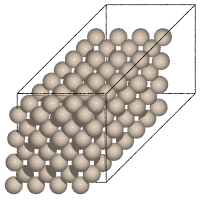
Mode #0

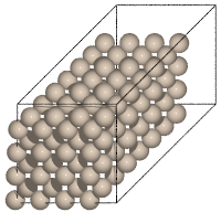
Mode #1

Mode #2

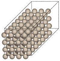
Optical vibration modes

Mode #3

Mode #4

Mode #5

We can clearly see that the atoms in bands 0, 1, and 2 moves in the same direction as a whole, while the atoms in bands 3, 4, and 5 vibrate against each other. Thus, three phonon branches with lower frequencies are acoustic branches, and the other three phonon branches are optical branches.

Transverse and Longitudinal branch

The phonon branches can also be grouped into transverse and longitudinal branches according to the direction of atom vibration and wave vector. In a transverse phonon mode, the atomic displacement is perpendicular to the wave vector \(\vec q\). In a longitudinal phonon mode, the atomic displacement is parallel to the wave vector \(\vec q\).

We can also determine whether the vibration mode is longitudinal or transverse from the following calculation.

reciprocal_basis = atoms.cell.reciprocal()
q_real = reciprocal_basis.dot(np.array([0.1, 0, 0]))

def get_angles(eigenvector, q_real):
    return np.arccos(eigenvector.dot(q_real) / np.linalg.norm(eigenvector, axis=1) / np.linalg.norm(q_real))

for i in range(6):
    angles = get_angles(eigenvector[i].real, q_real)
    print(f"Band {i}:")
    print(f"    Angles between q and eigenvectors:", angles)

Band 0:
    Angles between q and eigenvectors: [1.571 1.571]
Band 1:
    Angles between q and eigenvectors: [1.571 1.571]
Band 2:
    Angles between q and eigenvectors: [3.142 3.142]
Band 3:
    Angles between q and eigenvectors: [0.008 3.134]
Band 4:
    Angles between q and eigenvectors: [1.565 1.576]
Band 5:
    Angles between q and eigenvectors: [1.566 1.578]

We can see that \(\vec{q}\) and eigenvectors are parallel in bands 2 and 3, thus, they are longitudinal waves. On the contrary, \(\vec{q}\) and eigenvectors are perpendicular to each other in bands 0, 1, 4, and 5, and they are transverse waves.

In general, the 6 phonon branches of crystal silicon are:

• Transverse acoustic branch (TA): branches 0 and 1

• Longitudinal acoustic branch (LA): branch 2

• Transverse optic branch (TO): branches 4 and 5

• Longitudinal optic branch (LO): branch 3

2.6 Phonon density of state (DOS)

Phonon dispersion can provide insight into material properties; however, phonon dispersion is a non-trivial function in 3D and it is often helpful to bin modes by energy to simplify the description of what modes are present in a solid. As a consequence, we define the phonon density of states (DOS), which is the number of modes within \(\omega\) to \(\omega+d\omega\).

\[D(\omega) = \frac{1} {N} \sum_{m, \vec q} \delta (\omega - \omega_{m, \vec q})\]

Here, we use PostPhononDOSFeature to calculate the phonon DOS of crystal silicon

from matlantis_features.features.phonon import PostPhononDOSFeature, plot_band_dos

dos = PostPhononDOSFeature()
dos_results = dos(
    force_constant,
    kpts = [20,20,20],
    freq_min = -5.0,
    freq_max = 70.0,
    freq_bin =  1.0,
    scheme = "mp",
    unit = "meV"
)

from plotly.offline import iplot

fig = plot_band_dos(band_results, dos_results)
fig.update_layout(width=1000, height=500)
iplot(fig)

The phonon dispersion and phonon DOS are displayed together in the above figure. In the PostPhononDOSFeature, we calculate the phonon frequencies on a uniform mesh of \(\vec q\) points in the first Brillouin zone. Usually, the mesh grids can be the Monkhorst-Pack scheme or the Gamma-centered scheme. In the above example, a $20 \times `20 :nbsphinx-math:times 20 $ Monkhorst-Pack style grid is used. Please refer to the `appendix for the detailed explanation of Phonon DOS.

2.7 Thermochemistry properties

As we mentioned, the thermal property of a solid is closely related to phonon dispersion. Actually, as long as we know the phonon DOS, we can obtain several thermal properties, including specific heat \(C_V\), entropy \(S\), internal energy \(U\), and Helmholtz free energy \(A\).

The above properties are calculated with the following formula.

\[C_V = \int_{0}^{\infty} d {\omega} D(\omega) \; k_B\left( \frac{\hbar \omega}{k_B T} \right)^2 \frac{e^{\frac{\hbar \omega}{k_B T}}}{\left( e^{\frac{\hbar \omega}{k_B T}} - 1 \right)^2}\]

\[S = \int_{0}^{\infty} d {\omega} D(\omega) \; \left[ ln \left( \frac {1}{e^{\frac{\hbar \omega}{k_B T}}-1} + 1 \right ) \left( \frac {1}{e^{\frac{\hbar \omega}{k_B T}}-1} + 1 \right ) - ln \left( \frac {1}{e^{\frac{\hbar \omega}{k_B T}}-1} \right ) \left( \frac {1}{e^{\frac{\hbar \omega}{k_B T}}-1} \right ) \right]\]

\[U = \int_{0}^{\infty} d {\omega} D(\omega) \; \left[ \frac{\hbar \omega}{2} + \frac {\hbar \omega}{e^{\frac{\hbar \omega}{k_B T}} -1} \right]\]

\[A = \int_{0}^{\infty} d {\omega} D(\omega) \; \left[ \frac{\hbar \omega}{2} + k_BT ln \left( 1-e^{-\frac{\hbar \omega}{k_BT}} \right) \right]\]

[Note]

Phonon, which includes quantum effects, can only take discrete energies. It is known that phonon’s temperature dependency (quantum statistics) is different compared to classical lattice vibration. Due to this fact, Dirac constant \(\hbar\) appeared in the above equations.

We can simply use the PostPhononThermochemistryFeature in the Matlantis-Features package to do the above calculation. Simlar to the PostPhononDOSFeature, we should define the mesh of \(\vec q\) points. The PostPhononThermochemistryFeature will calculate the DOS from the force constant at first and then obtain the thermal properties according to the above formula.

from matlantis_features.features.phonon import PostPhononThermochemistryFeature

thermo = PostPhononThermochemistryFeature()
thermo_results = thermo(
    force_constant,
    kpts = [20, 20, 20],
    tmin = 0.0,
    tmax = 1000.0,
    tstep = 10.0,
    scheme = "mp",
)

import pandas as pd
import plotly.graph_objects as go

thermo_dft = pd.read_csv("../assets/Si_thermo_dft.csv")
thermo_expt = pd.read_csv("../assets/Si_thermo_expt.csv")

fig = thermo_results.plot()
fig.add_trace(
    go.Scatter(
        x = thermo_dft["T"].loc[:100],
        y = thermo_dft["entropy"].loc[:100] / 28.09 / 2.,
        name = "S DFT(J/K/g)"
    )
)
fig.add_trace(
    go.Scatter(
        x = thermo_dft["T"].loc[:100],
        y = thermo_dft["cv"].loc[:100] / 28.09 / 2.,
        name = "Cv DFT(J/K/g)"
    )
)
fig.add_trace(
    go.Scatter(
        x = thermo_dft["T"].loc[:100],
        y = thermo_dft["internal_energy"].loc[:100] / 28.09 / 2./1000.,
        name = "U DFT (kJ/g)"
    )
)
fig.add_trace(
    go.Scatter(
        x = thermo_dft["T"].loc[:100],
        y = thermo_dft["helmholtz_free_energy"].loc[:100] / 28.09 / 2./1000.,
        name = "F DFT(kJ/g)"
    )
)
fig.add_trace(
    go.Scatter(
        x = thermo_expt["T"],
        y = thermo_expt["cp"],
        mode = "markers",
        name = "Cp expt(J/k/g)"
    )
)
fig.add_trace(
    go.Scatter(
        x = thermo_expt["T"],
        y = thermo_expt["entropy"],
        mode = "markers",
        name = "S expt(J/k/g)"
    )
)
fig.update_layout(width=800, height=500)

The calculation result is plotted in the above figure. We can see the result agrees with the DFT and experiment results.

DFT calculation results from

A. Jain, S.P. Ong, G. Hautier, W. Chen, W.D. Richards, S. Dacek, S. Cholia, D. Gunter, D. Skinner, G. Ceder, K.A. Persson (*=equal contributions)

The Materials Project: A materials genome approach to accelerating materials innovation APL Materials, 2013, 1(1), 011002.

doi:10.1063/1.4812323

[bibtex]

Licensed under CC BY 4.0

Experiment results from

“Condensed Phase Heat Capacity Data” by Eugene S. Domalski and Elizabeth D. Hearing in NIST Chemistry WebBook, NIST Standard Reference Database Number 69, Eds. P.J. Linstrom and W.G. Mallard, National Institute of Standards and Technology, Gaithersburg MD, 20899, https://doi.org/10.18434/T4D303, (retrieved May, 2022).

3. Limitation of harmonic approximation

As shown in the above example, we can calculate the phonon dispersion, phonon DOS and some thermal properties of a crystal based on the harmonic approximation. However, such an approximation also hinders the application of phonon analysis in some physical properties since it totally ignores the anharmonicity of the potential energy surface. The most important two aspects are thermal expansion and thermal conductivity.

3.1 Thermal expansion

Thermal expansion can not be directly obtained from the phonon analysis. It is because the phonon calculation is based on the harmonic approximation, which assumes neighboring atoms are connected with perfect springs. In another word, the local potential energy surface is a quadratic function. But the real potential energy surface is actually not a quadratic function (please refer to Fig 1 in chapter 4.1). If two atoms are connected with the perfect spring, the bond length will not increase when the temperature is higher. Thus the volume of the solid will not increase with temperature. The thermal expansion is zero.

However, the thermal expansion can be calculated from the quasi-harmonic approximation. In the quasi-harmonic approximation, the phonon calculation is performed for a series of structures with compressed or stretched lattices. The volume-dependent properties, not only thermal expansion but also specific heat (Cp), Gibbs free energy (G), etc, can be obtained accordingly.

3.2 Thermal conductivity

Since the phonon carries energy and momentum. Thermal transportation can be explained as the movement of phonons in the crystal. However, since the phonon analysis is based on the harmonic approximation, the scattering between two phonons is ignored. In this case, one phonon can transport an infinitely long distance without collision with another phonon, which leads to infinite large thermal conductivity. As a consequence, we cannot get thermal conductivity from simple phonon calculation.

To consider the anharmonicity and phonon-phonon scattering, the third order Taylor series of potential energy should be considered.

\[E(\{\vec{R_{k}^{a}}\}) = E(\{\vec{R_{k,0}^{a}}\}) + \sum_{ak\alpha}{\sum_{bk'\beta}{\frac{1}{2} \left (\frac{\partial^2{E}}{\partial{u_{k}^{a\alpha}} \partial{u_{k'}^{b\beta}}} \right ) }} u_{k}^{a\alpha} u_{k'}^{b\beta} + \sum_{ak\alpha}{\sum_{bk'\beta} \sum_{ck''\gamma} {\frac{1}{3!} \left (\frac{\partial^3{E}}{\partial{u_{k}^{a\alpha}} \partial{u_{k'}^{b\beta}} \partial{u_{k''}^{c\gamma}}} \right ) }} u_{k}^{a\alpha} u_{k'}^{b\beta} u_{k''}^{c\gamma}\]

Thus, we should calculate the third order force constant, i.e. \(\frac{\partial^3{E}}{\partial{u_{k}^{a\alpha}} \partial{u_{k'}^{b\beta}} \partial{u_{k''}^{c\gamma}}}\). Several methods have been developed for the calculation of lattice thermal conductivity, such as real-time approximation.

4. References

[1] https://personales.unican.es/junqueraj/JavierJunquera_files/Metodos/Latticedynamics/Lattice-dynamics.pdf [2] http://www-personal.umich.edu/~sunkai/teaching/Winter_2013/chapter5.pdf [3] http://staff.ustc.edu.cn/~zqj/posts/LinearTetrahedronMethod/ [4] Otero-De-La-Roza, et. al. Comput. Phys. Commun. 182, 2232–2248 (2011). [5] “Introduction to Solid State Physics” Charles Kittel

5. Appendix

5.1 Formulations of phonon calculation

Illustration

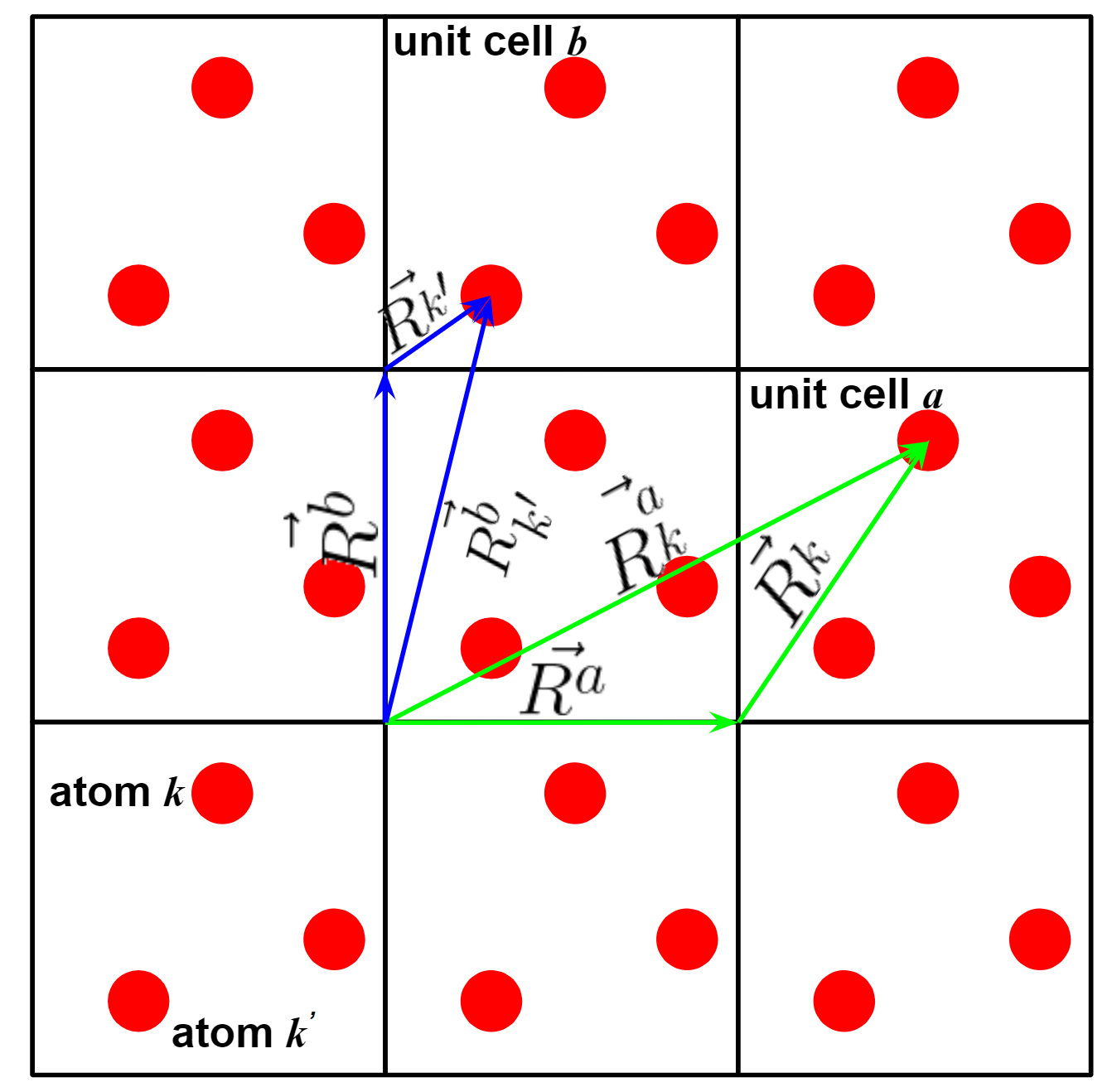
Before go to the formula deduction, we first show an 2D illustration of crystal structure. The meaning of several vectors in the figure is given as follow.

• \(\vec{R^{a}}\) the vector from original point of original unit cell to the original point of unit cell \(\mathit{a}\).

• \(\vec{R_{k}^{a}}\) the vector from original point of original unit cell to the atom \(\mathit{k}\) of unit cell \(\mathit{a}\).

• \(\vec{R_{k}}\) the vector from original point to the atom \(\mathit{k}\) in the same unit cell.

Harmonic approximation

• Similar to the vibration calculation, the potential energy of a system can be expressed as the following equation when atoms slightly deviated from the equilibrium position.

\[E(\{\vec{R_{k}^{a}}\}) = E(\{\vec{R_{k,0}^{a}}\}) + \sum_{ak\alpha}{\sum_{bk'\beta}{\frac{1}{2} \left (\frac{\partial^2{E}}{\partial{u_{k}^{a\alpha}} \partial{u_{k'}^{b\beta}}} \right ) }} u_{k}^{a\alpha} u_{k'}^{b\beta}\]

In this equation, \(\vec {u^a}\) is the displacement of an atoms from its equilibrium position \(\vec {R^a} - \vec {R_0^a}\), \(\alpha\) and \(\beta\) represent the cartesian directions, i.e. x, y and z.

• Please note that the harmonic approximation is valid only when atoms are slightly displaced from their equilibrium positions. That’s why we can only get the low-temperature thermal properties of crystal from phonon analysis.

Motion equation

• The force act on the atom \(\mathit{k}\) can be calculated from the derivative of the potential energy

\[\vec{F_{k}^{a\alpha}} = -\frac{E \left( \{R_{k}^{a} \} \right)}{\partial R_{k}^{a\alpha}} = -\frac{E \left( \{R_{k}^{a} \} \right)}{\partial u_{k}^{a\alpha}} = -\sum_{bk'\beta} \left ( \frac{\partial ^{2} E}{\partial{u_{k}^{a\alpha}} \partial{u_{k'}^{b\beta}}} \right ) u_{k'}^{b\beta}\]

• Acceleration of atom \(\mathit{k}\)

\[\vec{a_{k}^{a\alpha}} = \frac{\partial^2 u_{k}^{a\alpha}}{\partial t^2}\]

• So, the motion equation can be written as

\[M_k \frac{\partial^2 u_{k}^{a\alpha}}{\partial t^2} = -\sum_{bk'\beta} \left ( \frac{\partial ^{2} E}{\partial{u_{k}^{a\alpha}} \partial{u_{k'}^{b\beta}}} \right ) u_{k'}^{b\beta}\]

• There are 3 motion equations for each atom. In total, there are \(3N \times M\) equations for the system (\(N\) is the number of atoms in a unit cell, and \(M\) is the number of unit cells).

• The motion equations are coupled. The atomic displacement of the atom \(k\) in the \(a^{th}\) unit cell \(u_{k}^{a\alpha}(t)\) depends on the \(u_{k'}^{b\beta}\) of all the other atoms in the whole system.

Assumption

• To solve the above equations, we introduce two assumptions.

• 1. We assume that the \(u_{k}^{a\alpha}(t)\) has the following format.

     \[u_{k}^{a\alpha}(t) = A_{k}^{\alpha} e^{-i\omega t}\]

     Considering that the equation might have multiple solutions, we add the letter \(\mathit{m}\) as the index of different solutions.

\[u_{k}^{a\alpha}(t) = A_{k, m}^{\alpha} e^{-i\omega_{m} t} \;\;\; m={1, 2, ..., 3N}\]

• 2. Considering the periodical boundary condition, we assume the solution has a similar format to a plane wave, which is,

\[u_{k}^{a\alpha}(t) = A_{k, m \vec{q}}^{\alpha} e^{i \vec{q} \vec{R_a}} e^{-i\omega_{m} t}\]

• With the above assumptions, the solution of the motion equation depends on a new parameter \(\vec{q}\), which is the wavevector.

Solve the motion equation

• With the above assumptions, the motion equation can be written as

\[M_{k} \omega_{m\vec{q}}^{2} A_{m\vec{q}}^{k\alpha} = \sum_{k'\beta} {\left[ \sum_{b} {\left( \frac{\partial ^{2} E}{\partial{u_{k}^{a\alpha}} \partial{u_{k'}^{b\beta}}} \right) e^{i\vec{q}(\vec{R_b} - \vec{R_a})}} \right] A_{m\vec{q}}^{k'\beta}}\]

• Here, we define the force constant, which is a \(3N \times 3N\) matrix, in a similar way as that in vibration analysis. However, considering the periodical boundary condition, the force constant between the unit \(a\) and the unit \(b\) is represented as follows.

\[\begin{split}C^{a,b} = \begin{bmatrix} & \frac{\partial ^2 E}{\partial u_{0}^{a x} \partial u_{0}^{bx}} & \frac{\partial ^2 E}{\partial u_{0}^{a x} \partial u_{0}^{by}} & ... & \frac{\partial ^2 E}{\partial u_{0}^{a x} \partial u_{N}^{bz}} \\ & \frac{\partial ^2 E}{\partial u_{0}^{a y} \partial u_{0}^{bx}} & \frac{\partial ^2 E}{\partial u_{0}^{a y} \partial u_{0}^{by}} & ... & \frac{\partial ^2 E}{\partial u_{0}^{a y} \partial u_{N}^{bz}} \\ & ... & ... & & ...\\ & \frac{\partial ^2 E}{\partial u_{N}^{a z} \partial u_{N}^{bx}} & \frac{\partial ^2 E}{\partial u_{N}^{a z} \partial u_{0}^{by}} & ... & \frac{\partial ^2 E}{\partial u_{N}^{a z} \partial u_{N}^{bz}} \end{bmatrix}\end{split}\]

• Considering the translational invariance of the crystal lattice, the \(C^{a,b} = C^{0, b-a}\)

• In this case, the part between the brackets […] in the motion equation can be regarded as the discrete Fourier transform of the force constant in real space.

\[\tilde{C}_{\vec{q}}[k\alpha, k'\beta] = \sum_{b} {\left( \frac{\partial ^{2} E}{\partial{u_{k}^{a\alpha}} \partial{u_{k'}^{b\beta}}} \right) e^{i\vec{q}(\vec{R_b} - \vec{R_a})}} = \sum_{b} {C^{0,b}[k\alpha, k'\beta] e^{i\vec{q}(\vec{R_b} - \vec{R_a})}}\]

• To further simplify the motion equation, we define another \(3N \times 3N\) matrix called the dynamics matrix

\[\tilde{D}_{\vec{q}}[k\alpha, k'\beta] = \frac{1}{\sqrt{M_k M_{k'}}} \tilde{C}(\vec{q})[k\alpha, k'\beta]\]

• Then, the motion equation for the given \(q\) vector can be simplified as a linear homogenous system of equations

\[\boldsymbol{\tilde{D}_{\vec{q}}} \cdot \vec{\gamma}_{\vec{q}} = \omega^2_{\vec{q}} \vec{\gamma}_{\vec{q}}\]

where, the \(\vec{\gamma}_{\vec{q}}\) is called eigenvector, which is related to the amplitude of each atom by the following equation

\[A_{k, m \vec{q}}^{\alpha} = \frac{1}{\sqrt{M_k}} \gamma_{k, m\vec{q}}^{\alpha}\]

• Diagonlize the dynamical matrix \(\boldsymbol{\tilde{D}_{\vec{q}}}\), we can easily get the \(3N\) vibration frequencies \(\omega\) of the lattice for the given wave vector \(\vec{q}\).

5.2 Why \(\vec{q}\) is limited to the first Brillouin zone?

We will explain why the \(\vec{q}\) is limited in the first Brillouin zone using a simple 1D case. Essentially, this limitation originates from the discrete lattice points of the crystal atomic structure.

As we explained before, the atomic displacement of atom \(a\) in a 1D lattice should be

\[u_{q}^{a}(t) = A e^{i q x_a} e^{-i\omega_{m} t}\]

Suppose that the coordinate of atoms \(a\) is \(x=0.0\), and the lattice constant is 1.0. Then the reciprocal lattice point \(G \in (... -2\pi, 0, 2\pi, 4\pi, ...)\), and the first Brillouin zone is \([-\pi, \pi]\).

The following figure shows the \(u_{q}^{a}(t)\) when \(q\) is \(-\pi/3\) (blue line), \(-\pi/3+2\pi\) (green line) and \(-\pi/3+4\pi\) (yellow line). We can see that the displacement of atoms \(a\), which is indicated by the red dot, is exactly the same in the three waves.

\(u_{q}^{a}(t) = u_{q+G}^{a}(t)\)

In another word, for any \(\vec{q}\), there will be an equivalent \(\vec{q}'\) in the first Brillouin zone which has the same displacement of atoms \(u_{q}^{a}(t)\)

5.3 Phonon density of state and thermochemistry properties

Planck distribution

In a solid, there will be many phonons excited at the same time. To get the thermal properties from phonon analysis, it is important to understand the distribution of phonons. The energy of a phonon is given by \(E=\hbar\omega\). For a given phonon mode (fixed \(\vec q\) and \(\omega\)) the probability of having \(n\) phonons is \(P(n)=\frac{1}{Z}e^{-\frac{n\hbar\omega}{k_B T}}\), where \(Z\) is the normalization factor. So, the average number of phonons at a given temperature \(T\) can be expressed as

\[<n> = \sum_{0}^{\infty} {n P(n)} = \frac{1}{e^{\frac{\hbar\omega}{k_BT}}-1}\]

This is known as Planck distribution. The plot of Planck distribution is given below.

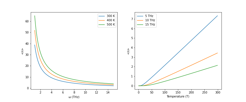
• From the left figure, we can see that the number of low-frequency phonons is much larger than that of high-frequency phonons, especially at the low temperature.

• From the right figure, we can see that the number of phonons will increase with the temperature.

• The total energy carried by the phonon with frequency \(\omega\) is simply obtained by:

  \[<E_{\omega}> = <n> \hbar \omega = \frac{\hbar \omega}{e^{\frac{\hbar \omega}{k_B T}}-1}\]

Phonon density of state

• One of the most important properties of a crystal system is its phonon density of states (DOS), which is defined by:

  \[D(\omega) = \frac{1} {N} \sum_{m, \vec q} \delta (\omega - \omega_{m, \vec q})\]

  in which, \(m\) is the band index, \(\vec q\) should walk through the first Brillouin zone. The DOS \(D(\omega)\) should follow the constraint

  \[N =\int_{0}^{\infty} D(\omega) d \omega\]

  in which \(N\) is the total number of phonon modes.

• If we know the density of states of phonon \(D(\omega)\), we can easily get the energy contribution from phonon

  \[U' = \int_{0}^{\infty} d {\omega} D(\omega) E_{\omega} = \int_{0}^{\infty} d {\omega} D(\omega) \; \left[ \frac{\hbar \omega}{2} + \frac {\hbar \omega}{e^{\frac{\hbar \omega}{k_B T}} -1} \right] = \int_{0}^{\infty} d {\omega} D(\omega) \frac{\hbar \omega}{e^{\frac{\hbar \omega}{k_B T}}-1}\]

  Note that the zero-point energy of a phonon, just like the quantum harmonic oscillator, is \(\frac {\hbar \omega}{2}\). If we include the zero point energy, the internal energy of a crystal can be expressed as

  \[U = \int_{0}^{\infty} d {\omega} D(\omega) \; \left[ \frac{\hbar \omega}{2} + \frac {\hbar \omega}{e^{\frac{\hbar \omega}{k_B T}} -1} \right]\]

• Many properties of the crystal can be related to the total internal energy \(U\). For example, the heat capacity \(C_V\) is

  \[C_V = \left( \frac{\partial U}{\partial T} \right)_V = \int_{0}^{\infty} d {\omega} D(\omega) Nk_B\left( \frac{\hbar \omega}{k_B T} \right)^2 \frac{e^{\frac{\hbar \omega}{k_B T}}}{\left( e^{\frac{\hbar \omega}{k_B T}} - 1 \right)^2}\]

• The specific heat \(C_V\), entropy \(S\), internal energy \(U\) and Helmholtz free energy \(A\) can be calculated from phonon DOS as well.

How to get phonon density of states

• From the above analysis, we can understand the many thermal properties that can be obtained from the phonon density of states. But, how can we get the phonon DOS?

• Firstly, we should calculate the phonon frequencies on a uniform mesh of \(\vec q\) points in the first Brillouin zone. Usually, the mesh grids can be the Monkhorst-Pack scheme or the Gamma-centered scheme.

• Then the phonon frequency is integrated over the first Brillouin zone. Usually, two methods can be used, the smearing method or the tetrahedral integral method

  • In the tetrahedron method, the mesh grids are divided into tetrahedra. Within each tetrahedral, the phonon frequency can be interpolated linearly. In this way, the phonon DOS can be obtained analytically. [3]

  • In the smearing method, the gaussian smearing function is added to all the phonon frequencies get from the mesh grid of \(\vec q\).