Appendix 1: Visualization
This section presents techniques on how to visualize atomic systems on Jupyter Notebook.
目次
ASE
save png image of atoms
save gif image of traj
nglviewer
ASE + nglviewer visualization
pfcc-extras
view_nglmethodIndex and position of each atom is visualized on tooltip
Save png, html
Show charge (Calculator required)
Show force (Calculator required)
nglviewer tips
Distance, angle, dihedral angle visualization with right click
povray
gif image visualization with povray
Other visualization tools
Utilizing VMD, OVITO
Preparation
Here is a case where one system atoms is visualized and another case where a time series traj is displayed.
First, prepare the atoms and traj to be visualized this time.
[1]:
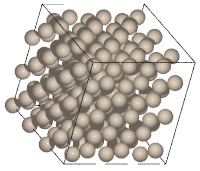
from ase.build import bulk

atoms = bulk("Si", cubic=True) * (3, 3, 3)

from ase.visualize import view
view(atoms, viewer="ngl")
[1]:
[2]:
from pfp_api_client.pfp.calculators.ase_calculator import ASECalculator
from pfp_api_client.pfp.estimator import Estimator, EstimatorCalcMode


estimator = Estimator(calc_mode=EstimatorCalcMode.PBE, model_version="v8.0.0")
calculator = ASECalculator(estimator)
[3]:
from ase.md.velocitydistribution import MaxwellBoltzmannDistribution, Stationary
from ase.md.verlet import VelocityVerlet
from ase.io import Trajectory
from ase import units

atoms.calc = calculator
# Set the momenta corresponding to T=500K.
MaxwellBoltzmannDistribution(atoms, temperature_K=5000.0)
# Sets the center-of-mass momentum to zero.
Stationary(atoms)
# Run MD using the VelocityVerlet algorithm
dyn = VelocityVerlet(atoms, 1.0 * units.fs, trajectory="output/dyn.traj")

def print_dyn():
    print(f"Dyn  step: {dyn.get_number_of_steps(): >3}, energy: {atoms.get_total_energy():.3f}")

dyn.attach(print_dyn, interval=10)
dyn.run(100)
Dyn  step:   0, energy: -847.935
Dyn  step:  10, energy: -847.842
Dyn  step:  20, energy: -847.837
Dyn  step:  30, energy: -847.867
Dyn  step:  40, energy: -847.854
Dyn  step:  50, energy: -847.846
Dyn  step:  60, energy: -847.849
Dyn  step:  70, energy: -847.847
Dyn  step:  80, energy: -847.850
Dyn  step:  90, energy: -847.852
Dyn  step: 100, energy: -847.844
[3]:
True
ASE
First, we will show you how to create png images and gif animations using the ASE built-in methods.
Using the write method, we can visualize and save the file in each format by specifying the extension “.png” for atoms or “.gif” for traj. Saved files can be visualized in Jupyter Notebook using IPython.display.Image.
[4]:
from ase.io import write
from IPython.display import Image
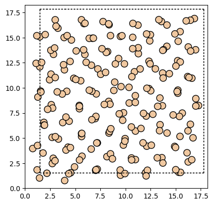
write("output/Si.png", atoms, rotation="0x,0y,0z")
Image(url="output/Si.png", width=300)
[4]:
You can rotate the displayed system by changing the value of rotation.
[5]:
write("output/Si_rotate_view.png", atoms, rotation="30x,30y,30z")
Image(url="output/Si_rotate_view.png", width=300)
[5]:
Trajectory traj, which consists of multiple atoms, can be animated to gif video by specifying “.gif” extension.
[6]:
traj = Trajectory("output/dyn.traj")
write("output/Si.gif", traj[::10], rotation="0x,0y,0z")
[7]:
Image(url="output/Si.gif", width=300)
[7]:
Image can be visualized or saved using matplotlib as well.
[8]:
import matplotlib.pyplot as plt
from ase.visualize.plot import plot_atoms

fig, ax = plt.subplots()
plot_atoms(atoms, ax, radii=0.3, rotation=("0x,0y,0z"))
fig.savefig("ase_slab.png")
For other details on ASE’s visualization methods, please refer to the following
nglviewer
It is also possible to display a 3D interactive system by using the library nglview.
There are several ways for visualization.
Method 1. using methods provided by nglview
The atoms can be displayed by using the show_ase method and the traj can be displayed by using the show_asetraj method.
If you add the gui=True option, a tab appears at the bottom where you can change various settings.
[9]:
import nglview as nv

nv.show_ase(atoms, gui=True)
[10]:
nv.show_asetraj(traj[::10], gui=True)
GUI style can be changed with gui_style.
[11]:
# v = nv.show_asetraj(traj[::10], gui=False)
# v.gui_style = "ngl"
# v
Executing above code shows the following
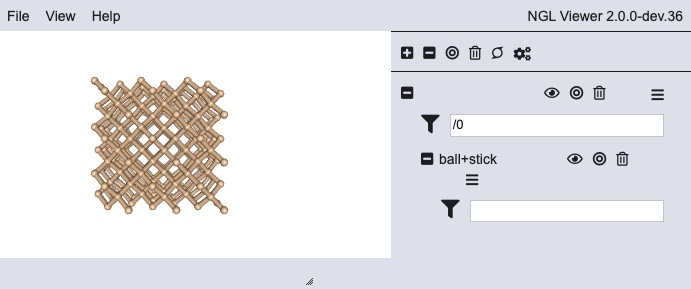
However, it is known to cause css styling problems when displaying this GUI style on the document in HTML. Thus a screenshot is shown here instead.
[12]:
v = nv.show_asetraj(traj[::10], gui=False)
v.add_representation("ball+stick")
v
Method 2: Using nglview via ASE’s viewer
It is also possible to display by specifying viewer="ngl" in the view method of ASE. You will see option to change some setting values on the right side in the ASE’s viewer.
[13]:
from ase.visualize import view

view(atoms, viewer="ngl")
[13]:
Same view method can be used for trajectory visualization.
[14]:
view(traj[::10], viewer="ngl")
[14]:
pfcc-extras
We provide pfcc-extras in Matlantis product, and viewer is provided with some additional customizations.
view_ngl method has following arguments
representations: NGL Viewer specific representations can be specified. One particularly common use case is to specify “ball+stick” to display the molecular bonds.w, h: NGL viewer width, height can be specified.
Some of the additional features:
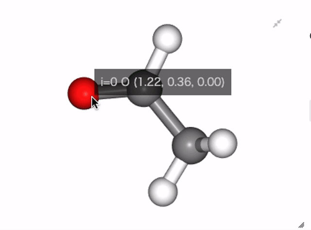
Index and position of each atom is visualized on tooltip
Save png, html
Show charge (Calculator necessary)
Show force (Calculator necessary)
[15]:
from pfcc_extras.visualize.view import view_ngl

view_ngl(atoms, representations=["ball+stick"], w=400, h=300)
[15]:
Tooltip to display index and positions of each atom
When you mouse over each atom, the index and the coordinates of each atom are displayed.
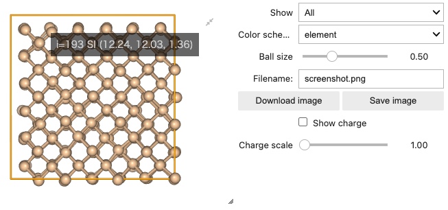
Support for save png, html format
“Download image” button downloads the currently displayed image to your PC. “Save image” button saves the currently displayed image to the current directory.
By default, it is “screenshot.png”, but you can also save it in HTML format by setting the extension to .html.
Show force (Calculator required)
By checking the “Show force” checkbox, you can visualize the force vector working on each atom. By changing the “Force scale”, you can change the size of the vector.
Note that calculator must be set for atoms.
[16]:
from ase.build import molecule
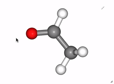
ch3cho_atoms = molecule("CH3CHO")
ch3cho_atoms.pop(0)
ch3cho_atoms.calc = calculator
view_ngl(ch3cho_atoms, representations=["ball+stick"], w=400, h=300, show_force=True)
[16]:
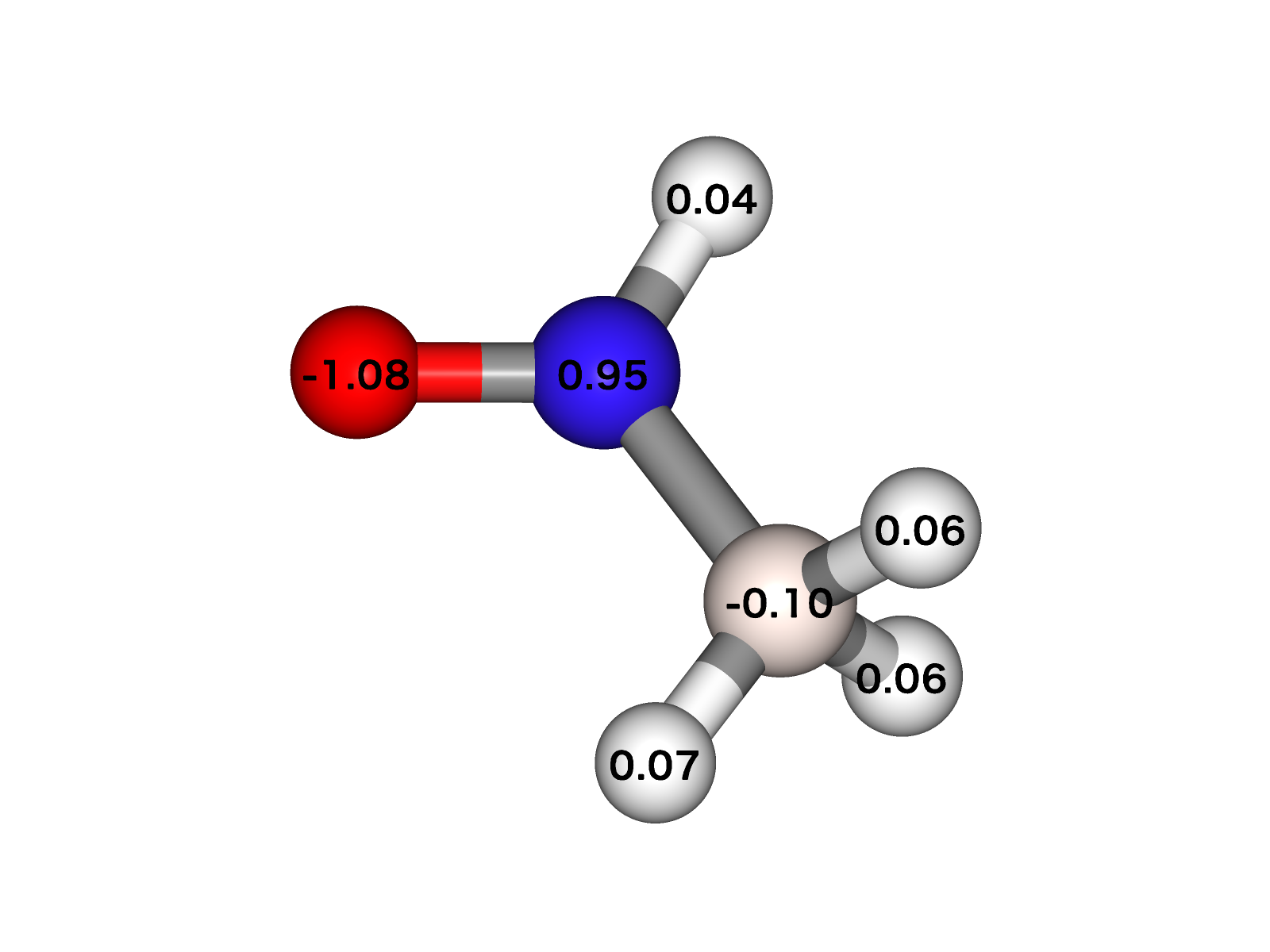
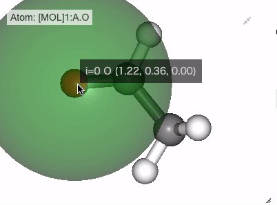
Show charge (Calculator required)
By checking the “Show charge” checkbox, you can visualize the charge of each atom. By changing the “Charge scale”, you can change the color shade.
Note that it is necessary to set calculator which can calculate charge for atoms.
[17]:
from ase.build import molecule

ch3cho_atoms = molecule("CH3CHO")
ch3cho_atoms.calc = calculator
view_ngl(ch3cho_atoms, representations=["ball+stick"], w=400, h=300)
[17]:
Charge value can be displayed using view.add_label method.
[18]:
v = view_ngl(ch3cho_atoms, representations=["ball+stick"], w=400, h=300)
v.gui.show_charge_checkbox.value = True
v.view.add_label(
    color="black", labelType="text",
    labelText=[f"{charge:.2f}" for charge in ch3cho_atoms.get_charges().ravel()],
    zOffset=1.0, attachment="middle_center", radius=0.5)
v
[18]:
Example:
replace_structure
In the default nglviewer, bond and cell are set for the very first atoms even when displaying trajectory. And only the coordinate values are updated when the frame is changed. Therefore, the
Bond changes (broken or connected)
Change in cell size
Increase/decrease of the number of atoms (ex. Evapolate or Deposit in LAMMPS)
Elemental species change
cannot be displayed.
Even in these cases, correct representation can be displayed by setting replace_structure=True as shown in the example below. (Note that this setting will slow down the display compared to the default setting, since calculations such as updating the bond display will be performed each time.)
[19]:
ch3cl_atoms = molecule("CH3Cl")

atoms_list = [ch3cl_atoms, ch3cho_atoms]
view_ngl(atoms_list, representations=["ball+stick"], replace_structure=True, w=400, h=300)
[19]:
nglviewer tips
Distance, angle and dihedral angle display on right click
In NGLViewer, you can press right-click to select an atom to measure and display the following values.
Distance: a right click on “atom 1” -> double right clicks on “atom 2”
Angle: a right click on “atom 1” -> a right click on “atom 2” -> double right clicks on “atom 3”
Dihedral Angle: a right click on “atom 1” -> a right click on “atom 2” -> a right click on “atom 3” -> double right clicks on “atom 4”
[20]:
view_ngl(ch3cho_atoms, representations=["ball+stick"], replace_structure=True, w=400, h=300)
[20]:
Example:
Show distance between atom 0 and 1
Show angle of atom 0, 1 and 2
Show dihedral angle of atom 0, 1, 2 and 3
povray
You can also use povray to visualize atomic systems.
With povray installed and the povray command available, you can create a gif image of the trajectory by executing the following method.
[21]:
from pfcc_extras.visualize.povray import traj_to_gif

traj_to_gif(
    traj[::10],
    gif_filepath="output/Si_anim.gif",
    povdir="output/pov",
    pngdir="output/png",
    clean=False
)
[Parallel(n_jobs=4)]: Using backend ThreadingBackend with 4 concurrent workers.
[Parallel(n_jobs=4)]: Done  11 out of  11 | elapsed:    6.8s finished
[22]:
Image("output/Si_anim.gif")
[22]:
<IPython.core.display.Image object>
[23]:
from pfcc_extras.visualize.povray import traj_to_apng

traj_to_apng(
    traj[::10],
    apng_filepath="output/Si_anim.png",
    povdir="output/pov",
    pngdir="output/png",
    clean=False
)
[Parallel(n_jobs=4)]: Using backend ThreadingBackend with 4 concurrent workers.
[Parallel(n_jobs=4)]: Done  11 out of  11 | elapsed:    6.8s finished
[24]:
Image("output/Si_anim.png")
[24]:
Using other visualization tools
If you wish to use another visualization tool, save the traj file in a different format. Here we convert to xyz, pdb files. These formats are accepted by the following tools.
For single system visualization, you can use
For trajectory visualization,
etc. may be used.
[25]:
from ase.io import write

# traj = Trajectory("output/dyn.traj")
write("output/si_traj.xyz", traj)
write("output/si_traj.pdb", traj)