Vibration Analysis
In the previous chapters, we have studied the various energies that can be obtained from locally stable structures.
In this chapter, we will look at the physical properties obtained by analyzing the curvature of the PES (Potential Energy Surface) around the local minimum.
First, let’s look at the vibration analysis for systems without periodic boundaries (e.g., organic molecules). The physical property obtained from the vibration analysis can be measured in reality with, such as IR spectra.
Harmonic approximation
Let us consider approximating the potential energy \(V\) around a local stable point, which we have obtained using Calculator.
The one-variable function \(f(x)\) around a given point \(x_0\) can be expressed as follows using the Taylor expansion
where \(\Delta x = x - x_0\).
Similarly, the multivariable function \(f(\mathbf{x})\) can be expressed as
where \(\Delta \mathbf{x} = \mathbf{x} - \mathbf{x_0}\).
Now, applying this equation to the potential energy \(V(\mathbf{r})\), at the point \(\mathbf{r_0}\) where the structure is stable. Since the force \(\mathbf{F}_i = \frac{\partial V(\mathbf{r_0})}{\partial r_i}\) is zero, the terms in the first derivative are zero. The expansion to the second order yields
The second derivative of energy, \(\frac{\partial^2 V(\mathbf{r_0})}{\partial r_i \partial r_j}\), is called Hessian or force constant matrix.
The potential energy surface that considers only second-order terms has the same energy as a system that is connected by springs, and thus, it is called the harmonic approximation.
The following example is shown in 5-9 harmonic approxmation – Shinshu Univ., Physical Chemistry Lab., Adsorption Group. The red line represents the Morse potential \(D(1-e^{- \beta x})^2\), and the blue line represents the harmonic oscillator potential \((1/2)kx^2\) centered at the stable point at \(x=0\). It can be seen that the approximation holds to some extent near \(x=0\).

Figure 1. Morse potential (red line) and harmonic oscillator potential (blue line) Cite from Shinshu Univ., Physical Chemistry Lab., Adsorption Group Iiyama & Futamura Laboratory.
Vibration
The potential energy \(V(\mathbf{r})\) is a \(3N\)-dimensional function for a system containing \(N\) atoms because each atom has three degrees of freedom in \(x, y, z\). Hence, Hessian \(\frac{\partial^2 V(\mathbf{r_0})}{\partial r_i \partial r_j}\) is a \(3N \times 3N\)-dimensional matrix. By diagonalizing the Hessian matrix, \(3N\) eigenvalues and eigenvectors are obtained.
Each eigenvalue corresponds to the strength of the spring \(k\) and each eigenvector corresponds to the direction of the spring, i.e. vibration mode. Among the \(3N\) degrees of freedom, there are 3 degrees of freedom that represent the translational motion of the entire molecule. In addition, the number of degrees of freedom for the rotation of the entire molecule around its center of mass is 2 for linear molecules and 3 for nonlinear molecules. Finally, The number of vibration modes (reference vibrations) is as follows after subtracting the translational and rotational degrees of freedom.
Linear molecule: \(3N-5\)
Nonlinear molecule: \(3N-6\)
Let’s look at examples. The Vibration module in ASE can be used to perform vibration analysis.
H2O
Since H2O is a nonlinear molecule consisting of three atoms, there should be six translational and rotational degrees of freedom and three vibration modes.
When performing a vibration analysis, we first optimize the structure of the system till the force is zero.
[1]:
from ase.build import molecule
from ase.optimize import LBFGS, BFGS, FIRE
import pfp_api_client
from pfp_api_client.pfp.calculators.ase_calculator import ASECalculator
from pfp_api_client.pfp.estimator import Estimator, EstimatorCalcMode

estimator = Estimator(calc_mode=EstimatorCalcMode.PBE, model_version="v8.0.0")
calculator = ASECalculator(estimator)
atoms = molecule("H2O")
atoms.calc = calculator
LBFGS(atoms).run(fmax=0.0001)
       Step     Time          Energy          fmax
LBFGS:    0 05:45:02      -10.057427        0.207265
LBFGS:    1 05:45:02      -10.058143        0.083642
LBFGS:    2 05:45:02      -10.058258        0.045952
LBFGS:    3 05:45:02      -10.058402        0.013669
LBFGS:    4 05:45:02      -10.058406        0.003253
LBFGS:    5 05:45:02      -10.058407        0.000200
LBFGS:    6 05:45:02      -10.058407        0.000008
[1]:
True
The vibration modes can be calculated with the Vibrations of ASE. In this module, Hessian is approximately calculated from the difference of the force when the position of the atom is slightly changed, as shown in the following equation.
Here, \(\Delta{r_i}\) is a vector that denotes the slight change of the ith coordinates. The vib.run() perform the above calculation and diagonalize Hessian, and vib.summary() outputs the square root of the eigenvalues.
The vib.run() creates the directory specified by name and caches the calculation results. Therefore, if a cache file remains when the next calculation is performed, the new calculation result will not be reflected. Cached files can be deleted with vib.clean().
[2]:
from ase.vibrations import Vibrations

vib = Vibrations(atoms, indices=None, delta=0.01, name="vib-h2o", nfree=2)
vib.clean()
vib.run()
vib.summary()
---------------------
  #    meV     cm^-1
---------------------
  0    6.3i     50.9i
  1    0.1i      0.6i
  2    0.0i      0.2i
  3    0.0i      0.1i
  4    3.3      26.5
  5    3.5      28.0
  6  194.7    1570.3
  7  459.0    3702.2
  8  471.3    3800.9
---------------------
Zero-point energy: 0.566 eV
The results show that the eigenenergies of the #0 to #5 modes, which actually correspond to translational and rotational modes, are almost zero. We also see that the eigenenergies of #6-#8 modes are greater than zero.
[Note]
The eighvalue with “i” are imaginary number. It indicates an upward convex quadratic form if we expressed the potential energy surface as a quadratic function. The existence of an imaginary eigenvalue suggests the existence of a point with even lower energy. It is caused by the undesirable behavior around the local stable point during structural optimization. However, this time the value is not large and can be regarded as almost zero.
Let’s look at each vibration mode.
Using vib.write_mode(), a trajectory file is created for each vibration mode under the current directory with the name specified by name.
[3]:
for i in range(len(vib.get_energies())):
    vib.write_mode(i)
In the following code, you can see how each vibration mode behaves by changing the value of mode from 0 to 8.
In fact, the values of mode from 0 to 5 indicate translational or rotational motion, while the values from 6 to 8 show that the vibration modes are described as follows.
mode 6: Vibration in which the angle of the H2O changes (bending vibration)
mode 7: Vibration in which the bond length between HOs changes simultaneously (symmetric stretch vibration)
mode 8: Vibration in which the bond lengths between HOs change alternately (asymmetric stretch vibration)
Each vibration can also be confirmed by IR spectra. You can also refer below for the reference.
[4]:
from ase.io.trajectory import Trajectory
from pfcc_extras.visualize.view import view_ngl

mode = 6
traj = Trajectory(f"vib-h2o.{mode}.traj")
view_ngl(traj, representations=["ball+stick"])
[4]:
You can also save each vibration mode as an animated png file as follows
[5]:
from tqdm.auto import tqdm
from pfcc_extras.visualize.povray import traj_to_apng


for mode in tqdm(range(9)):
    traj = Trajectory(f"vib-h2o.{mode}.traj")
    traj_to_apng(traj, f"output/vib-h2o.{mode}.png", rotation="90x,90y,180z", clean=True, n_jobs=16)
[Parallel(n_jobs=16)]: Using backend ThreadingBackend with 16 concurrent workers.
[Parallel(n_jobs=16)]: Done  30 out of  30 | elapsed:    2.4s finished
[Parallel(n_jobs=16)]: Using backend ThreadingBackend with 16 concurrent workers.
[Parallel(n_jobs=16)]: Done  30 out of  30 | elapsed:    2.5s finished
[Parallel(n_jobs=16)]: Using backend ThreadingBackend with 16 concurrent workers.
[Parallel(n_jobs=16)]: Done  30 out of  30 | elapsed:    2.7s finished
[Parallel(n_jobs=16)]: Using backend ThreadingBackend with 16 concurrent workers.
[Parallel(n_jobs=16)]: Done  30 out of  30 | elapsed:    2.3s finished
[Parallel(n_jobs=16)]: Using backend ThreadingBackend with 16 concurrent workers.
[Parallel(n_jobs=16)]: Done  30 out of  30 | elapsed:    2.6s finished
[Parallel(n_jobs=16)]: Using backend ThreadingBackend with 16 concurrent workers.
[Parallel(n_jobs=16)]: Done  30 out of  30 | elapsed:    2.3s finished
[Parallel(n_jobs=16)]: Using backend ThreadingBackend with 16 concurrent workers.
[Parallel(n_jobs=16)]: Done  30 out of  30 | elapsed:    2.4s finished
[Parallel(n_jobs=16)]: Using backend ThreadingBackend with 16 concurrent workers.
[Parallel(n_jobs=16)]: Done  30 out of  30 | elapsed:    2.5s finished
[Parallel(n_jobs=16)]: Using backend ThreadingBackend with 16 concurrent workers.
[Parallel(n_jobs=16)]: Done  30 out of  30 | elapsed:    2.4s finished
H2O vibration modes
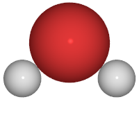
Mode #6
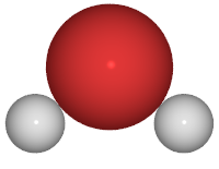
Mode #7
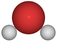
Mode #8
CO2
CO2 consists of the same three atoms as H2O, but is a linear molecule. Therefore, it is expected to have five translational and rotational modes and four vibration modes.
Let’s check it out here. As before, we will perform the structural optimization before the vibration analysis.
[6]:
atoms = molecule("CO2")
atoms.calc = calculator
LBFGS(atoms).run(fmax=0.001)
vib = Vibrations(atoms, indices=None, delta=0.01, name="vib-co2", nfree=2)
vib.clean()
vib.run()
vib.summary()
       Step     Time          Energy          fmax
LBFGS:    0 05:45:46      -17.747256        0.221567
LBFGS:    1 05:45:46      -17.747635        0.100589
LBFGS:    2 05:45:47      -17.747735        0.000831
---------------------
  #    meV     cm^-1
---------------------
  0    1.8i     14.9i
  1    1.8i     14.9i
  2    0.5i      4.0i
  3    1.0       7.8
  4    1.0       7.8
  5   70.3     567.2
  6   70.3     567.3
  7  163.6    1319.2
  8  289.5    2334.9
---------------------
Zero-point energy: 0.298 eV
[7]:
vib.write_mode()
In fact, the five modes corresponding to translation and rotation (#0-#4) have almost zero eigenenergy, while the eigenmodes corresponding to vibration (#5-#8) have values greater than zero.
Let us look at them. The vibration of #5 and #6 have the same eigenenergies, indicating that the vibration modes (= eigenvectors) are degenerate.
mode 5, 6: Vibrations that change the angle of CO2, showing degenerate changes in the two directions.
mode 7: Vibrations in which the bond lengths between the COs change simultaneously
mode 8: Vibrations in which the bond lengths between the COs change alternately.
[8]:
from ase.io.trajectory import Trajectory
from pfcc_extras.visualize.view import view_ngl

mode = 5
traj = Trajectory(f"vib-co2.{mode}.traj")
view_ngl(traj, representations=["ball+stick"])
[8]:
[9]:
from tqdm.auto import tqdm
from pfcc_extras.visualize.povray import traj_to_apng


for mode in tqdm(range(9)):
    traj = Trajectory(f"vib-co2.{mode}.traj")
    traj_to_apng(traj, f"output/vib-co2.{mode}.png", rotation="30x,30y,30z", clean=True, n_jobs=16)
[Parallel(n_jobs=16)]: Using backend ThreadingBackend with 16 concurrent workers.
[Parallel(n_jobs=16)]: Done  30 out of  30 | elapsed:    2.4s finished
[Parallel(n_jobs=16)]: Using backend ThreadingBackend with 16 concurrent workers.
[Parallel(n_jobs=16)]: Done  30 out of  30 | elapsed:    2.6s finished
[Parallel(n_jobs=16)]: Using backend ThreadingBackend with 16 concurrent workers.
[Parallel(n_jobs=16)]: Done  30 out of  30 | elapsed:    2.5s finished
[Parallel(n_jobs=16)]: Using backend ThreadingBackend with 16 concurrent workers.
[Parallel(n_jobs=16)]: Done  30 out of  30 | elapsed:    2.8s finished
[Parallel(n_jobs=16)]: Using backend ThreadingBackend with 16 concurrent workers.
[Parallel(n_jobs=16)]: Done  30 out of  30 | elapsed:    2.8s finished
[Parallel(n_jobs=16)]: Using backend ThreadingBackend with 16 concurrent workers.
[Parallel(n_jobs=16)]: Done  30 out of  30 | elapsed:    2.5s finished
[Parallel(n_jobs=16)]: Using backend ThreadingBackend with 16 concurrent workers.
[Parallel(n_jobs=16)]: Done  30 out of  30 | elapsed:    2.3s finished
[Parallel(n_jobs=16)]: Using backend ThreadingBackend with 16 concurrent workers.
[Parallel(n_jobs=16)]: Done  30 out of  30 | elapsed:    2.4s finished
[Parallel(n_jobs=16)]: Using backend ThreadingBackend with 16 concurrent workers.
[Parallel(n_jobs=16)]: Done  30 out of  30 | elapsed:    2.3s finished
CO2 vibration modes
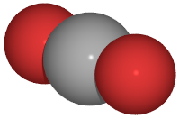
Mode #5
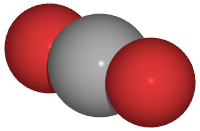
Mode #6
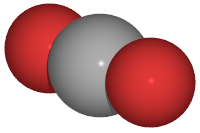
Mode #7

Mode #8
CH3OH
Let us go on to the same vibration analysis with CH3OH, a molecule with a slightly more complex shape.
Since it is a nonlinear molecule with six atoms, we see that the first six are translational and vibration modes, and the remaining 12 are vibration modes.
[10]:
atoms = molecule("CH3OH")
atoms.calc = calculator
LBFGS(atoms).run(fmax=0.001)
vib = Vibrations(atoms, indices=None, delta=0.01, name="vib-ch3oh", nfree=2)
vib.clean()
vib.run()
vib.summary()
       Step     Time          Energy          fmax
LBFGS:    0 05:46:25      -22.456031        0.265552
LBFGS:    1 05:46:25      -22.458848        0.160229
LBFGS:    2 05:46:25      -22.460468        0.072844
LBFGS:    3 05:46:25      -22.460642        0.067998
LBFGS:    4 05:46:25      -22.460903        0.025962
LBFGS:    5 05:46:25      -22.460962        0.020857
LBFGS:    6 05:46:26      -22.460994        0.017396
LBFGS:    7 05:46:26      -22.461026        0.017394
LBFGS:    8 05:46:26      -22.461047        0.009302
LBFGS:    9 05:46:26      -22.461054        0.008129
LBFGS:   10 05:46:26      -22.461057        0.006117
LBFGS:   11 05:46:26      -22.461057        0.007193
LBFGS:   12 05:46:26      -22.461058        0.003987
LBFGS:   13 05:46:26      -22.461058        0.001096
LBFGS:   14 05:46:26      -22.461063        0.000608
---------------------
  #    meV     cm^-1
---------------------
  0    1.5i     12.2i
  1    0.9i      7.3i
  2    0.1i      0.4i
  3    0.0       0.3
  4    0.1       0.7
  5    0.8       6.3
  6   37.3     300.5
  7  123.8     998.8
  8  129.9    1047.9
  9  139.7    1127.0
 10  163.7    1320.1
 11  176.1    1420.2
 12  179.1    1444.8
 13  180.3    1453.9
 14  361.0    2911.8
 15  367.1    2960.7
 16  376.9    3039.9
 17  463.4    3737.8
---------------------
Zero-point energy: 1.350 eV
Let’s take a look at each vibration mode. We can see that the whole atom moves in a complex manner for some vibration modes.
[11]:
vib.write_mode()
[12]:
from ase.io.trajectory import Trajectory
from pfcc_extras.visualize.view import view_ngl

mode = 10
traj = Trajectory(f"vib-ch3oh.{mode}.traj")
view_ngl(traj, representations=["ball+stick"])
[12]:
CH4
Finally, let us look at CH4 as an example of a molecule with high symmetry.
Since it is a nonlinear molecule with five atoms, we see that the first six are translational and rotational modes and the remaining nine are vibration modes.
[13]:
atoms = molecule("CH4")
atoms.calc = calculator
LBFGS(atoms).run(fmax=0.001)
vib = Vibrations(atoms, indices=None, delta=0.01, name="vib-ch4", nfree=2)
vib.clean()
vib.run()
vib.summary()
       Step     Time          Energy          fmax
LBFGS:    0 05:46:29      -18.196625        0.210110
LBFGS:    1 05:46:29      -18.198537        0.109506
LBFGS:    2 05:46:29      -18.199266        0.002115
LBFGS:    3 05:46:29      -18.199263        0.000019
---------------------
  #    meV     cm^-1
---------------------
  0    3.5i     28.3i
  1    3.5i     28.3i
  2    3.5i     28.3i
  3    0.3i      2.2i
  4    0.3i      2.2i
  5    0.3i      2.2i
  6  155.0    1250.3
  7  155.0    1250.3
  8  155.0    1250.3
  9  185.3    1494.6
 10  185.3    1494.6
 11  367.3    2962.5
 12  381.5    3076.9
 13  381.5    3076.9
 14  381.5    3076.9
---------------------
Zero-point energy: 1.174 eV
[14]:
vib.write_mode()
Physical properties calculated after vibration analysis
The following physical properties can be calculated by using the results of vibration analysis
Thermochemistry calculation: This method can be used to calculate enthalpy, free energy, etc. under the ideal gas approximation. Details are given in later chapters.
IR spectra wavenumber: Based on the vibrational analysis, we can identify the absorption wavenumbers of IR-active vibrational modes.
[Column] Effective range of harmonic approximation
Since the vibration analysis in this section and phonon analysis in the next section are based on the harmonic approximation, it is important to understand the structures and cases for which this approximation is valid. The harmonic approximation is based on the potential energy with spring \(1/2 k x^2\), to represent the potential energy near the stable structure. As shown in the figure below, the larger displacement of each atom from the origin, the larger force it will receive to pull it back to the origin. In other words, it is valid for structures such as solids, where the atoms stay in their positions, but not for fluids or gases, where each atom is not in a fixed place to begin with.
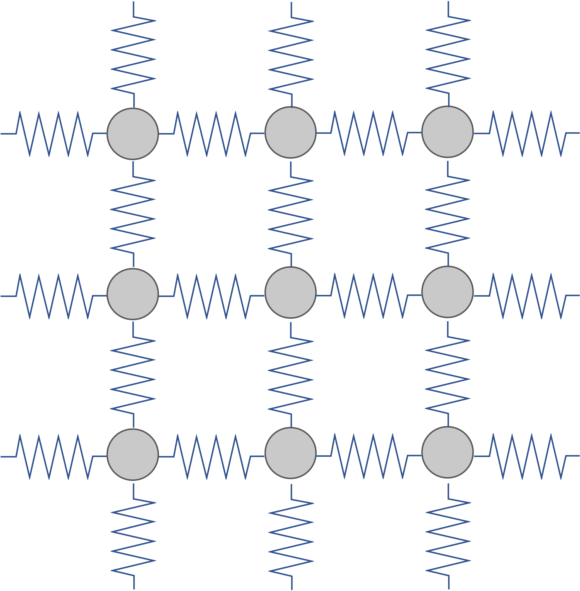
Diagram of an atomic system which the harmonic approximation is applied
This is also related to temperature. When a substance is above its melting point and in a liquid state, the harmonic approximation is not valid. As a rule of thumb, the accuracy of the harmonic oscillator approximation drops significantly as one approaches the melting point and it is only valid in the low temperature range.
Next section
In this section, we have performed vibration analysis for systems without periodic boundary conditions, such as molecules.
In the next section, we will deal with phonon, which describes vibration in a system with periodic boundary conditions, such as crystals.