Slab energy
We dealt with crystal structures (bulk) in the previous section.
As described later in chapter 5, we will deal with the reaction process of organic molecules on the surface of the catalyst metal when analyzing reactions on a catalyst. For this purpose, it is necessary to treat the structure on the surface of the material. In this section, we deal with the following energies related to the surface structure (referred to as “slab structure” in this Tutorial).
Surface energy
Interface energy
[1]:
from ase import Atoms
from ase.build import bulk
from ase.constraints import ExpCellFilter, StrainFilter
from ase.optimize import LBFGS, FIRE

import pfp_api_client
from pfp_api_client.pfp.calculators.ase_calculator import ASECalculator
from pfp_api_client.pfp.estimator import Estimator, EstimatorCalcMode


print(f"pfp_api_client: {pfp_api_client.__version__}")

estimator = Estimator(calc_mode=EstimatorCalcMode.PBE, model_version="v8.0.0")
calculator = ASECalculator(estimator)
pfp_api_client: 1.23.1
Surface energy
Surface energy is the energy required for a given crystal structure to create a surface, defined as the energy per unit area as follows.
\(E_{\rm{surface}}\) is the surface energy, \(E_{\rm{slab}}\) is the energy of the surface model described below, \(E_{\rm{bulk}}\) is the energy of the crystal, and \(A\) is the surface area of the upper and lower surfaces.
Surface energy of Pt111 surface
Let’s look at a concrete example to calculate the surface energy of the 111 surface of Pt metal with FCC structure. We will start with an explanation of the difference between the crystal structure and the slab structure (surface model).
[2]:
from ase.build import bulk, fcc111
from pfcc_extras.visualize.view import view_ngl


atoms_bulk = bulk("Pt", cubic=True) * (4, 4, 6)
atoms_slab = fcc111("Pt", size=(4, 4, 6), vacuum=10.0, orthogonal=True, periodic=True)
atoms_slab.pbc
[2]:
array([ True, True, True])
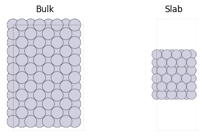
As shown in the figure below, the crystal structure is one in which the periodic boundary condition continues in the three-dimensional direction, while the slab (surface structure) is one in which the periodic boundary condition continues in only two directions in the xy-plane, but the surface is cut out in the z-direction.
However, when dealing with periodic boundary conditions in DFT calculations, etc., it is necessary to impose periodic boundary conditions in all three directions, so for modeling purposes, a “sufficiently large” cell size in the z-axis direction is used to represent the surface structure in a pseudo-surface manner. The required cell size along the z-axis depends on the force field chosen and should be kept to a level where the effect of the interaction of atoms above and below the z-axis is negligible. In the case of the PFP used here, the cutoff radius is 6A, so the vacuum layer (designated by the vacuum in the following) should be larger than 6A. When using quantum chemical calculations such as DFT, the larger the vacuum layer, the longer the calculation time may be, so it is necessary to select the appropriate size.
Here the fcc111 method is used with periodic=True, otherwise, the periodic boundary condition would be pbc=[True, True, False] and imposed only on the xy-plane. The vacuum layer is explicitly specified with vacuum argument, and the periodic boundary is imposed in all 3-dimensional directions.
[3]:
from ase.io import write
from IPython.display import Image
import matplotlib.pyplot as plt
import matplotlib.image as mpimg

write("output/pt_bulk.png", atoms_bulk, rotation="90x,0y,0z")
write("output/pt_slab.png", atoms_slab, rotation="90x,0y,0z")


fig, axes = plt.subplots(1, 2, figsize=(6, 3))
ax0, ax1 = axes
ax0.imshow(mpimg.imread("output/pt_bulk.png"))
ax0.set_axis_off()
ax0.set_title("Bulk")
ax1.imshow(mpimg.imread("output/pt_slab.png"))
ax1.set_axis_off()
ax1.set_title("Slab")
fig.show()
Surface modeling
Surfaces are in a completely different state than the interior of bulk. Even the basic property, coordination number (the number of atoms around each atom), is very different. As a result, the surface is generally unstable.
When creating a slab structure, it must be thick enough to represent the transition from the stable bulk state to the unstable surface state. In this example, six layers are taken in the z-axis direction. For this Tutorial, we recommend a minimum thickness of 4-6 layers.
The larger the thickness, the closer to reality the modeling will be. But when performing quantum chemical calculations, about 4 layers are often used due to limitations imposed by computation time.
In the xy-direction, the structure continues indefinitely due to the periodic boundary condition. For adsorption structures such as those described below, the supercell must be sufficiently large in the xy direction as well, but for surface energy, it can be small.
[4]:
view_ngl([atoms_slab, atoms_bulk], replace_structure=True)
[4]:
First, we perform structural optimization of the crystal structure to obtain E_bulk.
[5]:
symbol = "Pt"
atoms_bulk = bulk(symbol, "fcc")
atoms_bulk.calc = calculator
atoms_bulk_strain = StrainFilter(atoms_bulk, mask=[1, 1, 1, 0, 0, 0])
opt = LBFGS(atoms_bulk_strain)
#opt = BFGS(atoms_bulk_strain)
opt.run(fmax=0.001)
E_bulk = atoms_bulk.get_total_energy()
print(f"E_bulk = {E_bulk} eV")
/tmp/ipykernel_7549/2836453991.py:4: FutureWarning: Import StrainFilter from ase.filters
  atoms_bulk_strain = StrainFilter(atoms_bulk, mask=[1, 1, 1, 0, 0, 0])
       Step     Time          Energy          fmax
LBFGS:    0 04:11:41       -5.458319        1.594600
LBFGS:    1 04:11:41       -5.475224        0.023110
LBFGS:    2 04:11:41       -5.475228        0.003489
LBFGS:    3 04:11:41       -5.475231        0.000026
E_bulk = -5.475231107012031 eV
Next, the slab structure is created, and structural optimization is performed to obtain E_slab.
The cell size of the slab structure is fixed at the size obtained from the structural optimization result of the bulk structure. The structural optimization of the slab optimizes only the coordinate values.
The reason is that the slab structure is small for modeling purposes, but in reality, we want to consider the surface with respect to the infinitely large bulk structure, in which case the cell sizes in the x and y directions are expected to remain the same with bulk.
[6]:
a = atoms_bulk.cell[0, 2] * 2
atoms_slab = fcc111("Pt", size=(4, 4, 8), a=a, vacuum=40.0, periodic=True)
atoms_slab.calc = calculator
# atoms_slab_strain = ExpCellFilter(atoms_slab)
atoms_slab_strain = atoms_slab
opt = LBFGS(atoms_slab_strain)
#opt = BFGS(atoms_slab_strain)
opt.run(fmax=0.001)
E_slab = atoms_slab.get_total_energy()
print(f"E_slab = {E_slab} eV")
       Step     Time          Energy          fmax
LBFGS:    0 04:11:42     -680.730208        0.177141
LBFGS:    1 04:11:42     -680.748609        0.134948
LBFGS:    2 04:11:42     -680.773735        0.021800
LBFGS:    3 04:11:42     -680.774318        0.020075
LBFGS:    4 04:11:42     -680.774742        0.009221
LBFGS:    5 04:11:42     -680.774894        0.007406
LBFGS:    6 04:11:42     -680.774928        0.008192
LBFGS:    7 04:11:42     -680.775059        0.006255
LBFGS:    8 04:11:42     -680.775160        0.005650
LBFGS:    9 04:11:42     -680.775145        0.005372
LBFGS:   10 04:11:42     -680.775356        0.006000
LBFGS:   11 04:11:42     -680.775290        0.006580
LBFGS:   12 04:11:42     -680.775353        0.007512
LBFGS:   13 04:11:42     -680.775542        0.005780
LBFGS:   14 04:11:43     -680.775512        0.002725
LBFGS:   15 04:11:43     -680.775525        0.000546
E_slab = -680.7755252731672 eV
We have obtained E_bulk and E_slab.
The surface area \(A\) of the slab structure can be obtained as follows
[7]:
import numpy as np

cx, cy, cz = atoms_slab.cell
print("Cell length = ", cx, cy, cz)
A = np.linalg.norm(np.cross(cx, cy))

print(f"Area A = {A:.2f} A^2")
Cell length =  [11.23080333  0.          0.        ] [5.61540166 9.72616099 0.        ] [ 0.          0.         96.04734691]
Area A = 109.23 A^2
Finally, the surface energy \(E_{\rm{surface}}\) is calculated as follows. The denominator is \(2*A\) because there are two surfaces, one above and one below the z-axis.
[8]:
E_surface = (E_slab - E_bulk * len(atoms_slab) / len(atoms_bulk)) / (2 * A)
print(f"E_surface = {E_surface:.3f} eV/A^2")
E_surface = 0.092 eV/A^2
Surface energies of various metal 111 surfaces
Let us perform the above calculations for various metal atoms.
[9]:
from ase.optimize import BFGS

def get_opt_energy(atoms, fmax=0.001, opt_mode: str = "normal"):
    if opt_mode == "scale":
        opt = LBFGS(StrainFilter(atoms, mask=[1, 1, 1, 0, 0, 0]), logfile=None)
    elif opt_mode == "all":
        opt = LBFGS(UnitCellFilter(atoms), logfile=None)
    else:
        opt = LBFGS(atoms, logfile=None)
    opt.run(fmax=fmax)
    return atoms.get_total_energy()


def calc_fcc111_surface_energy(calculator, symbol: str = "Pt", size=(2, 4, 4)):
    atoms_bulk = bulk(symbol, "fcc")
    atoms_bulk.calc = calculator
    E_bulk = get_opt_energy(atoms_bulk, fmax=0.001, opt_mode="scale")
    a = atoms_bulk.cell[0, 2] * 2

    # Default pbc is [True, True, False] (not periodic on z-axis). But this is not supported in PFP so set all pbc=True.
    slab = fcc111(symbol, size=size, a=a, vacuum=40.0, periodic=True)
    slab.calc = calculator
    E_slab = get_opt_energy(slab, fmax=0.001)

    # calc area of slab on xy plane
    cx, cy, cz = slab.cell
    A = np.linalg.norm(np.cross(cx, cy))
    N = len(slab)
    E_surface = (E_slab - E_bulk * N) / (2 * A)  # unit (ev/A^2)
    print(f"E_slab {E_slab:.3f} eV, E_bulk {E_bulk:.3f} eV, E_surface {E_surface:.3f} eV/A^2, A {A} A^2, N {N}")
    return E_surface
Because of the faster computation time when using PFP, the following calculations are performed with 8 layers of thickness in the z-axis direction.
[10]:
E_surface_list = []
for symbol in ["Al", "Cu", "Rh", "Pd", "Ag", "Pt", "Au"]:
    E_surface = calc_fcc111_surface_energy(calculator, symbol, size=(4, 4, 8))
    print(f"{symbol} E_surface = {E_surface:.3f} eV/A^2")
    E_surface_list.append({"symbol": symbol, "E_surface[eV/A^2]": E_surface})
/tmp/ipykernel_7549/1216418715.py:5: FutureWarning: Import StrainFilter from ase.filters
  opt = LBFGS(StrainFilter(atoms, mask=[1, 1, 1, 0, 0, 0]), logfile=None)
E_slab -427.809 eV, E_bulk -3.441 eV, E_surface 0.056 eV/A^2, A 113.39021406367881 A^2, N 128
Al E_surface = 0.056 eV/A^2
E_slab -434.262 eV, E_bulk -3.508 eV, E_surface 0.081 eV/A^2, A 90.81951019513978 A^2, N 128
Cu E_surface = 0.081 eV/A^2
E_slab -712.057 eV, E_bulk -5.770 eV, E_surface 0.131 eV/A^2, A 101.53550955769842 A^2, N 128
Rh E_surface = 0.131 eV/A^2
E_slab -460.619 eV, E_bulk -3.739 eV, E_surface 0.083 eV/A^2, A 107.6094390054786 A^2, N 128
Pd E_surface = 0.083 eV/A^2
E_slab -311.226 eV, E_bulk -2.515 eV, E_surface 0.045 eV/A^2, A 119.32742776331231 A^2, N 128
Ag E_surface = 0.045 eV/A^2
E_slab -680.775 eV, E_bulk -5.475 eV, E_surface 0.092 eV/A^2, A 109.23269191647253 A^2, N 128
Pt E_surface = 0.092 eV/A^2
E_slab -377.557 eV, E_bulk -3.032 eV, E_surface 0.044 eV/A^2, A 119.7047752118272 A^2, N 128
Au E_surface = 0.044 eV/A^2
[11]:
import pandas as pd
df = pd.DataFrame(E_surface_list)
df
[11]:
| symbol | E_surface[eV/A^2] | |
|---|---|---|
| 0 | Al | 0.055857 |
| 1 | Cu | 0.081195 |
| 2 | Rh | 0.130776 |
| 3 | Pd | 0.083424 |
| 4 | Ag | 0.044542 |
| 5 | Pt | 0.091795 |
| 6 | Au | 0.043802 |
As shown above, we were able to determine the surface energies of various elements. If you want to convert units, for example, from eV/A^2 to J/m^2, you can calculate as follows
[12]:
from ase.units import J

# 1 Angstrom = 10^-10 meter
meter = 10 ** 10
ratio = J/(meter ** 2)
df["E_surface[J/m^2]"] = df["E_surface[eV/A^2]"] / ratio
df
[12]:
| symbol | E_surface[eV/A^2] | E_surface[J/m^2] | |
|---|---|---|---|
| 0 | Al | 0.055857 | 0.894924 |
| 1 | Cu | 0.081195 | 1.300889 |
| 2 | Rh | 0.130776 | 2.095255 |
| 3 | Pd | 0.083424 | 1.336608 |
| 4 | Ag | 0.044542 | 0.713648 |
| 5 | Pt | 0.091795 | 1.470722 |
| 6 | Au | 0.043802 | 0.701787 |
In the literature below, Cu 0.080, Pt 0.084, and Au 0.050 eV/A^2 are reported, which is close to our result.
Surface reconstruction
In the above calculations, the surface energy was obtained by structural optimization of the slab structure with a particular plane cut as it is, but it is known that the surface state of some materials can change significantly. For example, it is known that the (100) surface of silicon changes to a dimer structure and becomes stable. In such a case, it is necessary to calculate the structural relaxation taking the surface reconstruction into account, and optimization with the bulk-cut surface as it may result in high energy.
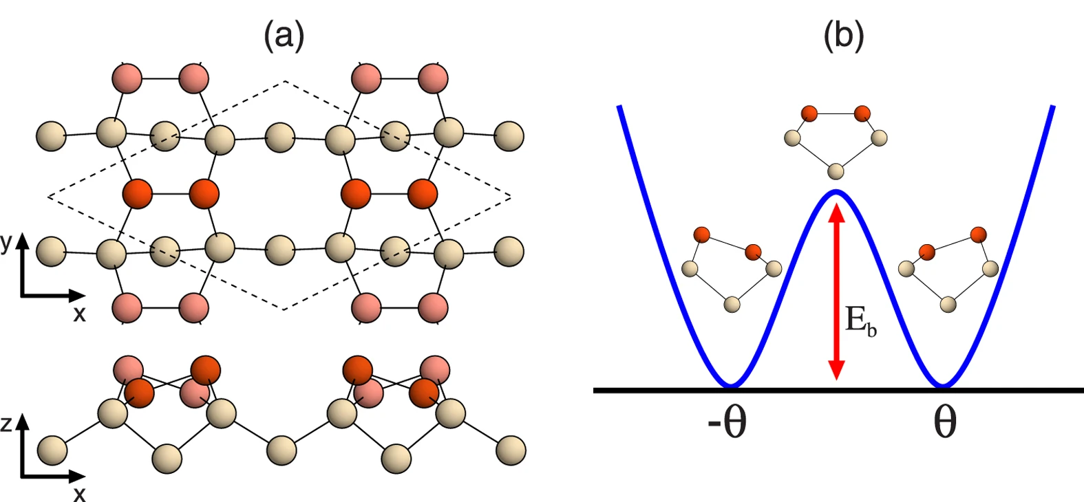
Figure 1 of “Origin of Symmetric Dimer Images of Si(001) Observed by Low-Temperature Scanning Tunneling Microscopy” (Licensed under CC BY 4.0)
Reference
Relaxation and reconstruction on (111) surfaces of Au, Pt, and Cu
「機械・材料設計に生かす 実践分子動力学シミュレーション」 泉 聡志・増田裕寿
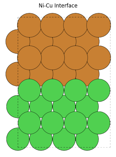
Interface energy
The junction surface of two different materials A and B is called the interface, and the energy required to create the interface is called the interface energy.
\(E^{AB}_{\rm{interface}}\) is the energy of the interface model jointing A and B, and \(E^{A}_{\rm{bulk}}, E^{B}_{\rm{bulk}}\) is the energy of the crystal structure of A and B, respectively. By looking at the interface energy, we can analyze whether substances A and B are a good combination to bond or not.
Interface energy calculations are in progress.
Here we present only a sample script for creating the interfacial structure to give you an idea of what the interfacial structure looks like.
In practice, several considerations are necessary
How to set the degree of distortion of substances A and B
Preliminary structural relaxation in the z-axis direction for each substance
For more details, please refer to the references as well.
[13]:
from ase.build import bulk, fcc111, fcc100
from pfcc_extras.visualize.view import view_ngl

a = 3.56
s = 4

cu_slab = fcc100("Cu", a=a, size=(s, s, s), vacuum=a/4, orthogonal=True, periodic=True)
ni_slab = fcc100("Ni", a=a, size=(s, s, s), vacuum=a/4, orthogonal=True, periodic=True)

# print(cu_slab, ni_slab)
view_ngl([cu_slab, ni_slab], replace_structure=True)
[13]:
[14]:
from pfcc_extras.visualize.ase import view_ase_atoms

_cu_slab = cu_slab.copy()
_ni_slab = ni_slab.copy()
_ni_slab.positions[:, 2] += cu_slab.cell[2, 2]

cu_ni_interface = _cu_slab + _ni_slab
cu_ni_interface.cell[2, 2] = ni_slab.cell[2, 2] + cu_slab.cell[2, 2]
[15]:
view_ase_atoms(cu_ni_interface, rotation="90x", figsize=(6, 6), scale=40, title="Ni-Cu Interface")
[16]:
view_ngl(cu_ni_interface)
[16]:
Reference
「機械・材料設計に生かす 実践分子動力学シミュレーション」 泉 聡志・増田裕寿