In the previous section, we learned how to use the NEB method to calculate activation energies using organic molecules as the example. In this section, we will try to analyze the reaction of NO dissociation on the heterogeneous catalyst Rh as a more practical application.
The workflow is as follows. Create the Rh slab structure that will be the catalyst. and adsorb the NO which is the reactant molecule. Then, the states before and after the reaction are created and the activation energy is calculated using the NEB method.
Note that the content of this tutorial is based on the example published in matlantis-contrib.
The sort method in ASE sorts the order of atoms according to the atomic number.
[3]:
frompfcc_extras.visualize.viewimportview_nglbulk=bulk.repeat([2,2,2])bulk=sort(bulk)# Shift positions a bit to prevent surface to be cut at wrong place when `makesurface` is calledbulk.positions+=[0.01,0,0]view_ngl(bulk,representations=["ball+stick"])
Create slab structures from bulk structures with any Miller index. We can specify the miller_indices=(x,y,z). The surface method is used in the makesurface to create a surface structure.
slab=makesurface(bulk,miller_indices=(1,1,1),layers=2,rep=[1,1,1])slab=sort(slab)# adjust `positions` before `wrap`slab.positions+=[1,1,0]slab.wrap()view_ngl(slab,representations=["ball+stick"])
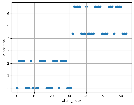
Check the highest coordinates of the slab along the z axis (it is necessary when creating the adsorption structure). Check the coordinates of each layer of the slab (it is necessary to determine how many layers to fix).
[6]:
importplotly.expressaspx# Check z_position of atomsatoms=slabdf=pd.DataFrame({"x":atoms.positions[:,0],"y":atoms.positions[:,1],"z":atoms.positions[:,2],"symbol":atoms.symbols,})display(df)coord="z"df_sorted=df.sort_values(coord).reset_index().rename({"index":"atom_index"},axis=1)fig=px.scatter(df_sorted,x=df_sorted.index,y=coord,color="symbol",hover_data=["x","y","z","atom_index"])fig.show()
Let’s create an adsorption structure. Here we use the add_adsorbate method to place the molec on top of the slab.
[16]:
mol_on_slab=slab.copy()# height: height of molecule from slab surface# position: x,y position of molecule# The molecule position can be modified later, and thus rough value is ok here.add_adsorbate(mol_on_slab,molec,height=3,position=(8,4))c=FixAtoms(indices=[atom.indexforatominmol_on_slabifatom.position[2]<=1])mol_on_slab.set_constraint(c)
The class SurfaceEditor is used to adjust the adsorption position of the molecule.
Use SurfaceEditor(atoms).display() to display the structure you want to edit.
Get the indices of the molecule you want to move with atomsz> button. The molecule is the atoms above the highest coordinate of the slab structure which we confirmed in 1-3. If set appropriately, only the index of the molecule will be included in the box below.
Use XYZ+- of “move”, “rotate” to change the position or the orientation of the molecule. Adjusting the ball size will make the adsorption site easier to be seen.
Click the “Run mini opt” button to perform the structural optimization using BFGS for a given number of steps.
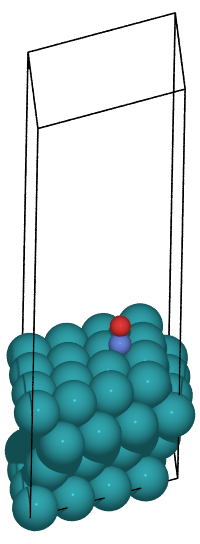
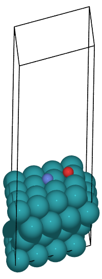
In this tutorial, we will create an adsorption structure based on the following paper.
“First-Principles Microkinetic Analysis of NO + CO Reactions on Rh(111) Surface toward Understanding NOx Reduction Pathways”
In this example, The hcp adsorption structure can be created by pressing “X-” three times, “Y+” once, and “Z-” four times. See the figure below for the FCC and HCP sites of adsorption.
The adsorption energy can be obtained by calculating the energy difference of the slab and the molecule when they existed separately and when they were combined.
The value in the above paper is 1.79 eV. The discrepancy is likely due to the fact that the paper uses the RPBE functional, while the PFP uses the PBE functional.
Here we will create the IS and FS structures to run the NEB. You may skip to 3. NEB calculation as we will use the structures we have created in advance.
This time, we will use the initial and final state files created in advance to perform the reaction path search. The example matlantis-contrib/matlantis_contrib_examples/NEB_Solid_catalyst shows the NEB calculation for the reaction NO(fcc) -> N(fcc) + O(fcc). In this Tutorial, we will try the NEB calculation for the reaction NO(fcc) -> N(hcp) + O(hcp).
IS -383.1211239113131 eV
FS -383.93783990736733 eV
[37]:
beads=21
NEB is faster with parallel=True and allowed_shared_calculator=False.
[38]:
b0=IS.copy()b1=FS.copy()configs=[b0.copy()foriinrange(beads-1)]+[b1.copy()]forconfiginconfigs:# Calculator must be set separately with NEB parallel=True, allowed_shared_calculator=False.estimator=Estimator(calc_mode=EstimatorCalcMode.CRYSTAL_PLUS_D3,model_version="v8.0.0")calculator=ASECalculator(estimator)config.calc=calculator
First, linear interpolation of configs, which are candidate reaction pathways, is performed using NEB interpolate method.
[39]:
# k: spring constant. It was stable to when reduced to 0.05neb=NEB(configs,k=0.05,parallel=True,climb=True,allow_shared_calculator=False)neb.interpolate()
/tmp/ipykernel_4043/1063292405.py:2: FutureWarning:
Please import NEB from ase.mep, not ase.neb.
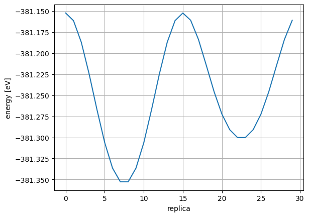
Check reaction path candidate after linear interpolation
It is recommended that fmax is 0.05 or less. If fmax is too small, it will take a long time to converge. We use a loose convergence condition (e.g., 0.2) in the first NEB calculation. If a reasonable reaction path is obtained, you can make the convergence condition tighter for a more stable calculation. If an abnormal reaction path is obtained with a loose convergence condition, please check the IS and FS structures.
The calculation time is around ten minutes. Please wait. Refer to neb_log.txt if you want to check the progress.
[42]:
%%timesteps=2000relax=FIRE(neb,trajectory=None,logfile=filepath+"/neb_log.txt")# fmax<0.05 recommended. It takes time when it is smaller.# 1st NEB calculation can be executed with loose condition (Ex. fmax=0.2),# and check whether reaction path is reasonable or not.# If it is reasonable, run 2nd NEB with tight fmax condition.# If the reaction path is abnormal, check IS, FS structure.relax.run(fmax=0.1,steps=steps)
CPU times: user 6.26 s, sys: 2.05 s, total: 8.31 s
Wall time: 14.1 s
[42]:
True
After the first loose convergence, check for anomalies in the reaction path.
[Parallel(n_jobs=4)]: Using backend ThreadingBackend with 4 concurrent workers.
[Parallel(n_jobs=4)]: Done 21 out of 21 | elapsed: 8.2s finished
[47]:
<IPython.core.display.Image object>
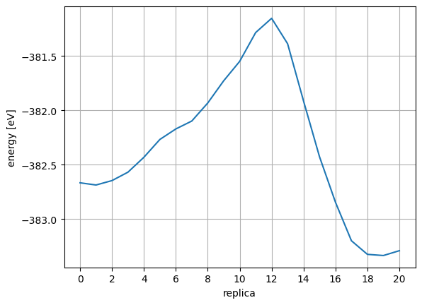
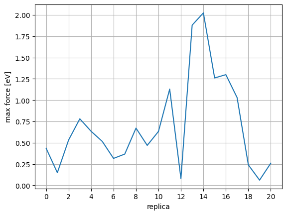
Obtain the index of TS structure. Looking at the energy and force, you can see that the system reaches the saddle point (see below) at index=12 where the energy is maximum and the force is near 0.
defcalc_max_force(atoms):return((atoms.get_forces()**2).sum(axis=1).max())**0.5mforces=[calc_max_force(config)forconfiginconfigs]plt.plot(range(len(mforces)),mforces)plt.xlabel("replica")plt.ylabel("max force [eV]")plt.xticks(np.arange(0,len(mforces),2))plt.grid(True)plt.show()
It should be confirmed in the max force plot that the force is close to 0 at the following three points:
Starting state (index=0)
Transition state (index=12)
End state (index=20)
However, we use FixAtoms to fix some atoms in this calculation. The points in the plot will not be 0 if the force of the fixed atoms is large.
The activation energy can be calculated by looking at the energy difference between the initial structure index=0 and the transition state index=12.
If the intermediate images obtained from NEB calculation contain a structure that is more suitable for the initial state and final state, please extract the structure and rerun the NEB using it as IS or FS.
5. Structural optimization of the transition state structure by Sella
The TS structure obtained in the NEB above is not the exact saddle point. (*) Here, the TS structure is optimized using a library called sella.
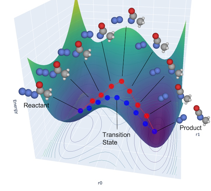
(*) What is saddle point:
The initial and final states are structures at local minima. Since the energy increases when a small displacement occurs in any direction, all components should be positive when the Hessian is diagonalized, as explained in section 4-1 Vibration (the second derivative is a positive definite matrix, and the intuitive explanation is that the energy surface looks like \(y=ax^2 (a>0)\) for any direction.).
In contrast, a transition state is one in which only one diagonal component of the Hessian is negative and the remaining components are positive (except 5 or 6 translational, rotational invariant direction). The energy goes down only in the direction connecting the initial state and the final state (in the shape of \(y=ax^2 (a<0)\) at the local potential energy surface), and the energy increases in the other directions. Such a point is called a saddle point.
See also the following figure used in the previous section.
To calculate the exact activation energy, it is necessary to find the exact transition state point.
[51]:
!pipinstallsella
Looking in indexes: https://pypi.org/simple, http://pypi.artifact.svc:8080/simple
Requirement already satisfied: sella in /home/jovyan/.py311/lib/python3.11/site-packages (2.3.5)
Requirement already satisfied: numpy>=1.14.0 in /home/jovyan/.py311/lib/python3.11/site-packages (from sella) (1.26.4)
Requirement already satisfied: scipy>=1.1.0 in /home/jovyan/.py311/lib/python3.11/site-packages (from sella) (1.15.3)
Requirement already satisfied: ase>=3.18.0 in /home/jovyan/.py311/lib/python3.11/site-packages (from sella) (3.25.0)
Requirement already satisfied: jax>=0.4.20 in /home/jovyan/.py311/lib/python3.11/site-packages (from sella) (0.6.2)
Requirement already satisfied: jaxlib>=0.4.20 in /home/jovyan/.py311/lib/python3.11/site-packages (from sella) (0.6.2)
Requirement already satisfied: matplotlib>=3.3.4 in /home/jovyan/.py311/lib/python3.11/site-packages (from ase>=3.18.0->sella) (3.10.3)
Requirement already satisfied: ml_dtypes>=0.5.0 in /home/jovyan/.py311/lib/python3.11/site-packages (from jax>=0.4.20->sella) (0.5.1)
Requirement already satisfied: opt_einsum in /home/jovyan/.py311/lib/python3.11/site-packages (from jax>=0.4.20->sella) (3.4.0)
Requirement already satisfied: contourpy>=1.0.1 in /home/jovyan/.py311/lib/python3.11/site-packages (from matplotlib>=3.3.4->ase>=3.18.0->sella) (1.3.2)
Requirement already satisfied: cycler>=0.10 in /home/jovyan/.py311/lib/python3.11/site-packages (from matplotlib>=3.3.4->ase>=3.18.0->sella) (0.12.1)
Requirement already satisfied: fonttools>=4.22.0 in /home/jovyan/.py311/lib/python3.11/site-packages (from matplotlib>=3.3.4->ase>=3.18.0->sella) (4.58.2)
Requirement already satisfied: kiwisolver>=1.3.1 in /home/jovyan/.py311/lib/python3.11/site-packages (from matplotlib>=3.3.4->ase>=3.18.0->sella) (1.4.8)
Requirement already satisfied: packaging>=20.0 in /home/jovyan/.py311/lib/python3.11/site-packages (from matplotlib>=3.3.4->ase>=3.18.0->sella) (25.0)
Requirement already satisfied: pillow>=8 in /home/jovyan/.py311/lib/python3.11/site-packages (from matplotlib>=3.3.4->ase>=3.18.0->sella) (11.2.1)
Requirement already satisfied: pyparsing>=2.3.1 in /home/jovyan/.py311/lib/python3.11/site-packages (from matplotlib>=3.3.4->ase>=3.18.0->sella) (3.2.3)
Requirement already satisfied: python-dateutil>=2.7 in /home/jovyan/.py311/lib/python3.11/site-packages (from matplotlib>=3.3.4->ase>=3.18.0->sella) (2.9.0.post0)
Requirement already satisfied: six>=1.5 in /home/jovyan/.py311/lib/python3.11/site-packages (from python-dateutil>=2.7->matplotlib>=3.3.4->ase>=3.18.0->sella) (1.17.0)
[notice] A new release of pip is available: 24.0 -> 25.1.1[notice] To update, run: pip install --upgrade pip
The transition state must be a saddle point where only one second derivative is negative and the others are positive. If more than one value is negative, it suggests the existence of the other transition states with lower activation energies than that point.
We will perform a vibrational analysis to make sure that we obtain the correct transition state.
[56]:
# Vibration analysis is executed with atoms `z_pos >= zz`z_pos=pd.DataFrame({"z":TS.positions[:,2],"symbol":TS.symbols,})vibatoms=z_pos[z_pos["z"]>=7.0].indexvibatoms
[56]:
Index([64, 65], dtype='int64')
[57]:
# Vibration analysisvibpath=filepath+"/TS_vib/vib"os.makedirs(vibpath,exist_ok=True)# Vibration analysis is executed with only specified atoms `indices=vibatoms`vib=Vibrations(TS,name=vibpath,indices=vibatoms)vib.run()vib_energies=vib.get_energies()thermo=IdealGasThermo(vib_energies=vib_energies,potentialenergy=potentialenergy,atoms=TS,geometry='linear',#'monatomic', 'linear', or 'nonlinear'symmetrynumber=2,spin=0,natoms=len(vibatoms),ignore_imag_modes=True)G=thermo.get_gibbs_energy(temperature=298.15,pressure=101325.)
Enthalpy components at T = 298.15 K:
===============================
E_pot -381.853 eV
E_ZPE 0.034 eV
Cv_trans (0->T) 0.039 eV
Cv_rot (0->T) 0.026 eV
Cv_vib (0->T) 0.005 eV
(C_v -> C_p) 0.026 eV
-------------------------------
H -381.724 eV
===============================
Entropy components at T = 298.15 K and P = 101325.0 Pa:
=================================================
S T*S
S_trans (1 bar) 0.0022653 eV/K 0.675 eV
S_rot 0.0012595 eV/K 0.376 eV
S_elec 0.0000000 eV/K 0.000 eV
S_vib 0.0000236 eV/K 0.007 eV
S (1 bar -> P) -0.0000011 eV/K -0.000 eV
-------------------------------------------------
S 0.0035474 eV/K 1.058 eV
=================================================
Free energy components at T = 298.15 K and P = 101325.0 Pa:
=======================
H -381.724 eV
-T*S -1.058 eV
-----------------------
G -382.781 eV
=======================