Slab + mol energy
Various processes are handled during reactions on catalysts, for example
Organic molecules are adsorbed on the catalyst surface
Reaction proceeds on the surface
After the reaction is completed, the product is desorbed from the catalyst surface
Since reactants and products adsorb and desorb on the catalyst, it is necessary to deal with adsorption structures (structures in which molecules exist on the surface structure).
In this section, we introduce the adsorption energy, the energy associated with the adsorption structure.
Adsorption energy
[1]:
from ase import Atoms
from ase.build import bulk
from ase.constraints import ExpCellFilter, StrainFilter
from ase.optimize import LBFGS, FIRE
import pfp_api_client
from pfp_api_client.pfp.calculators.ase_calculator import ASECalculator
from pfp_api_client.pfp.estimator import Estimator, EstimatorCalcMode
print(f"pfp_api_client: {pfp_api_client.__version__}")
estimator = Estimator(calc_mode=EstimatorCalcMode.PBE, model_version="v8.0.0")
calculator = ASECalculator(estimator)
pfp_api_client: 1.23.1
Adsorption energy
The adsorption energy \(E_{\rm{adsorption}}\) represents the energy difference before and after a molecule is adsorbed on a surface structure.
where \(E_{\rm{slab}}\) is the energy of the slab alone, \(E_{\rm{mol}}\) is the energy of the molecule alone, and \(E_{\rm{slab+mol}}\) is the energy of the adsorption structure with the molecule attached to the slab.
CO on Co
[2]:
from ase.optimize import LBFGS
from ase.build import fcc111, hcp0001, molecule, add_adsorbate
from ase.constraints import ExpCellFilter, StrainFilter
def get_opt_energy(atoms, fmax=0.001, opt_mode: str = "normal"):
atoms.set_calculator(calculator)
if opt_mode == "scale":
opt1 = LBFGS(StrainFilter(atoms, mask=[1, 1, 1, 0, 0, 0]))
elif opt_mode == "all":
opt1 = LBFGS(ExpCellFilter(atoms))
else:
opt1 = LBFGS(atoms)
opt1.run(fmax=fmax)
return atoms.get_total_energy()
First, the Co structure is prepared using the bulk, and the appropriate cell size is found by optimizing the cell size.
[3]:
bulk_atoms = bulk("Co")
bulk_atoms.cell
[3]:
Cell([[2.51, 0.0, 0.0], [-1.255, 2.173723763498941, 0.0], [0.0, 0.0, 4.07122]])
[4]:
bulk_atoms = bulk("Co")
bulk_atoms.calc = calculator
E_bulk = get_opt_energy(bulk_atoms, fmax=1e-4, opt_mode="scale")
E_bulk
Step Time Energy fmax
LBFGS: 0 05:00:53 -10.266314 0.917135
LBFGS: 1 05:00:53 -10.271767 0.190536
/tmp/ipykernel_3433/1344539460.py:7: FutureWarning: Please use atoms.calc = calc
atoms.set_calculator(calculator)
/tmp/ipykernel_3433/1344539460.py:9: FutureWarning: Import StrainFilter from ase.filters
opt1 = LBFGS(StrainFilter(atoms, mask=[1, 1, 1, 0, 0, 0]))
LBFGS: 2 05:00:53 -10.272057 0.065210
LBFGS: 3 05:00:54 -10.272109 0.007636
LBFGS: 4 05:00:54 -10.272111 0.000729
LBFGS: 5 05:00:54 -10.272112 0.000031
[4]:
-10.272111651260108
[5]:
bulk_atoms.cell
[5]:
Cell([[2.500496479864743, 0.0, 0.0], [-1.2502482399323716, 2.165493486666698, 0.0], [0.0, 0.0, 4.022806887309025]])
[6]:
# Set lattice parameter from bulk cell
a = bulk_atoms.cell[0,0]
c = bulk_atoms.cell[2,2]
a,c
[6]:
(2.500496479864743, 4.022806887309025)
You can see a slight change in value from the ASE default of a = 2.51A. We will use this cell size to create the adsorption structure below.
[7]:
slab = hcp0001("Co", size=(4, 4, 4), a=a, c=c, vacuum=40.0, periodic=True)
slab.calc = calculator
[8]:
E_slab = get_opt_energy(slab, fmax=1e-4, opt_mode="normal")
Step Time Energy fmax
LBFGS: 0 05:00:54 -304.787566 0.465494
/tmp/ipykernel_3433/1344539460.py:7: FutureWarning: Please use atoms.calc = calc
atoms.set_calculator(calculator)
LBFGS: 1 05:00:54 -304.910147 0.370066
LBFGS: 2 05:00:54 -305.125230 0.054862
LBFGS: 3 05:00:54 -305.127507 0.037520
LBFGS: 4 05:00:54 -305.128856 0.039435
LBFGS: 5 05:00:54 -305.133149 0.032470
LBFGS: 6 05:00:54 -305.135449 0.017488
LBFGS: 7 05:00:54 -305.136081 0.006170
LBFGS: 8 05:00:54 -305.136162 0.000781
LBFGS: 9 05:00:54 -305.136161 0.000038
[9]:
mol = molecule("CO")
mol.calc = calculator
E_mol = get_opt_energy(mol, fmax=1e-4)
Step Time Energy fmax
LBFGS: 0 05:00:55 -11.443040 0.797117
LBFGS: 1 05:00:55 -11.431574 1.878720
/tmp/ipykernel_3433/1344539460.py:7: FutureWarning: Please use atoms.calc = calc
atoms.set_calculator(calculator)
LBFGS: 2 05:00:55 -11.445926 0.046015
LBFGS: 3 05:00:55 -11.445934 0.002568
LBFGS: 4 05:00:55 -11.445933 0.000001
Creating adsorption structures
Adsorption structures can be created by using the add_adsorbate method to place molecules on the slab.
[10]:
%%time
slab_mol = hcp0001("Co", size=(4, 4, 4), a=a, c=c, vacuum=40.0, periodic=True)
mol2 = molecule("CO")
add_adsorbate(slab_mol, mol2, 3.0, "bridge")
E_slab_mol = get_opt_energy(slab_mol, fmax=1e-2)
Step Time Energy fmax
LBFGS: 0 05:00:55 -317.298055 3.367191
LBFGS: 1 05:00:55 -317.432694 4.081281
/tmp/ipykernel_3433/1344539460.py:7: FutureWarning: Please use atoms.calc = calc
atoms.set_calculator(calculator)
LBFGS: 2 05:00:55 -317.699263 2.858175
LBFGS: 3 05:00:55 -317.973910 1.086529
LBFGS: 4 05:00:55 -317.996378 0.707769
LBFGS: 5 05:00:55 -318.071190 0.641089
LBFGS: 6 05:00:55 -318.081374 0.367003
LBFGS: 7 05:00:55 -318.087663 0.250177
LBFGS: 8 05:00:56 -318.107622 0.845603
LBFGS: 9 05:00:56 -318.115923 0.647254
LBFGS: 10 05:00:56 -318.121235 0.170493
LBFGS: 11 05:00:56 -318.123992 0.213722
LBFGS: 12 05:00:56 -318.127948 0.427355
LBFGS: 13 05:00:56 -318.130845 0.379397
LBFGS: 14 05:00:56 -318.132463 0.151676
LBFGS: 15 05:00:56 -318.133156 0.059567
LBFGS: 16 05:00:56 -318.133794 0.175820
LBFGS: 17 05:00:56 -318.134569 0.215512
LBFGS: 18 05:00:56 -318.135123 0.130339
LBFGS: 19 05:00:57 -318.135360 0.023292
LBFGS: 20 05:00:57 -318.135485 0.049542
LBFGS: 21 05:00:57 -318.135621 0.088976
LBFGS: 22 05:00:57 -318.135744 0.078587
LBFGS: 23 05:00:57 -318.135825 0.030664
LBFGS: 24 05:00:57 -318.135852 0.010856
LBFGS: 25 05:00:57 -318.135869 0.030200
LBFGS: 26 05:00:57 -318.135916 0.038714
LBFGS: 27 05:00:57 -318.135927 0.024988
LBFGS: 28 05:00:58 -318.135928 0.007101
CPU times: user 162 ms, sys: 11.7 ms, total: 174 ms
Wall time: 2.7 s
[11]:
E_adsorp = E_slab_mol - (E_slab + E_mol)
print(f"E_adsorp {E_adsorp}, E_slab_mol {E_slab_mol}, E_slab {E_slab}, E_mol {E_mol}")
E_adsorp -1.5538343284925418, E_slab_mol -318.13592752018087, E_slab -305.13616061153743, E_mol -11.445932580150906
An adsorption energy of -1.55 eV was obtained.
[12]:
from pfcc_extras.visualize.view import view_ngl
view_ngl(slab_mol)
[12]:
Adsorption sites
You can specify the adsorption site name instead of the coordinate value as the fourth positional argument to the add_adsorbate method.
[13]:
%%time
slab_mol = hcp0001("Co", size=(4, 4, 4), a=a, c=c, vacuum=40.0, periodic=True)
mol2 = molecule("CO")
add_adsorbate(slab_mol, mol2, 3.0, "ontop")
E_slab_mol = get_opt_energy(slab_mol, fmax=1e-4)
Step Time Energy fmax
LBFGS: 0 05:01:04 -317.842476 2.898523
/tmp/ipykernel_3433/1344539460.py:7: FutureWarning: Please use atoms.calc = calc
atoms.set_calculator(calculator)
LBFGS: 1 05:01:04 -317.970380 3.594472
LBFGS: 2 05:01:04 -318.191337 1.677113
LBFGS: 3 05:01:05 -318.281429 0.675248
LBFGS: 4 05:01:05 -318.291021 0.402380
LBFGS: 5 05:01:05 -318.298278 0.037047
LBFGS: 6 05:01:05 -318.299164 0.060696
LBFGS: 7 05:01:05 -318.302288 0.184594
LBFGS: 8 05:01:05 -318.304052 0.160634
LBFGS: 9 05:01:05 -318.304860 0.053985
LBFGS: 10 05:01:05 -318.305023 0.024048
LBFGS: 11 05:01:05 -318.305066 0.019796
LBFGS: 12 05:01:05 -318.305139 0.025298
LBFGS: 13 05:01:05 -318.305123 0.013126
LBFGS: 14 05:01:05 -318.305191 0.004591
LBFGS: 15 05:01:05 -318.305180 0.004789
LBFGS: 16 05:01:05 -318.305185 0.009711
LBFGS: 17 05:01:06 -318.305189 0.010454
LBFGS: 18 05:01:06 -318.305212 0.005977
LBFGS: 19 05:01:06 -318.305179 0.001660
LBFGS: 20 05:01:06 -318.305149 0.002807
LBFGS: 21 05:01:06 -318.305150 0.003268
LBFGS: 22 05:01:06 -318.305208 0.002356
LBFGS: 23 05:01:06 -318.305210 0.001274
LBFGS: 24 05:01:06 -318.305172 0.001606
LBFGS: 25 05:01:06 -318.305206 0.002345
LBFGS: 26 05:01:06 -318.305210 0.002209
LBFGS: 27 05:01:06 -318.305215 0.001226
LBFGS: 28 05:01:06 -318.305168 0.000541
LBFGS: 29 05:01:06 -318.305219 0.000799
LBFGS: 30 05:01:07 -318.305208 0.000816
LBFGS: 31 05:01:07 -318.305170 0.000546
LBFGS: 32 05:01:07 -318.305226 0.000258
LBFGS: 33 05:01:07 -318.305159 0.000331
LBFGS: 34 05:01:07 -318.305154 0.000510
LBFGS: 35 05:01:07 -318.305206 0.000436
LBFGS: 36 05:01:07 -318.305153 0.000187
LBFGS: 37 05:01:07 -318.305170 0.000142
LBFGS: 38 05:01:07 -318.305219 0.000121
LBFGS: 39 05:01:07 -318.305208 0.000160
LBFGS: 40 05:01:07 -318.305180 0.000097
CPU times: user 217 ms, sys: 25.6 ms, total: 243 ms
Wall time: 3.08 s
The name of this adsorption site can be found by checking the “sites” in the .info attribute.
[14]:
slab_mol.info
[14]:
{'adsorbate_info': {'cell': array([[2.50049648, 0. ],
[1.25024824, 2.16549347]]),
'sites': {'ontop': (0, 0),
'bridge': (0.5, 0),
'fcc': (0.3333333333333333, 0.3333333333333333),
'hcp': (0.6666666666666666, 0.6666666666666666)},
'top layer atom index': 48}}
The “fcc111”, in this example, has ontop, bridge, fcc, and hcp sites Let’s take a look at each of them.
[15]:
orthogonal = False
slab_mol_ontop = hcp0001("Co", a=a, c=c, size=(4, 4, 4), vacuum=40.0, periodic=True, orthogonal=orthogonal)
mol = molecule("CO")
add_adsorbate(slab_mol_ontop, mol, 3.0, "ontop")
slab_mol_bridge = hcp0001("Co", a=a, c=c, size=(4, 4, 4), vacuum=40.0, periodic=True, orthogonal=orthogonal)
mol = molecule("CO")
add_adsorbate(slab_mol_bridge, mol, 3.0, "bridge")
slab_mol_fcc = hcp0001("Co", a=a, c=c, size=(4, 4, 4), vacuum=40.0, periodic=True, orthogonal=orthogonal)
mol = molecule("CO")
add_adsorbate(slab_mol_fcc, mol, 3.0, "fcc")
slab_mol_hcp = hcp0001("Co", a=a, c=c, size=(4, 4, 4), vacuum=40.0, periodic=True, orthogonal=orthogonal)
mol = molecule("CO")
add_adsorbate(slab_mol_hcp, mol, 3.0, "hcp")
[16]:
view_ngl([slab_mol_ontop, slab_mol_bridge, slab_mol_fcc, slab_mol_hcp])
[16]:
[17]:
from ase.io import write
from IPython.display import Image
import matplotlib.pyplot as plt
import matplotlib.image as mpimg
write("output/co_ontop.png", slab_mol_ontop, rotation="0x,0y,90z")
write("output/co_bridge.png", slab_mol_bridge, rotation="0x,0y,90z")
write("output/co_fcc.png", slab_mol_fcc, rotation="0x,0y,90z")
write("output/co_hcp.png", slab_mol_hcp, rotation="0x,0y,90z")
fig, axes = plt.subplots(1, 4, figsize=(12, 3))
for i, adsorbate_name in enumerate(["ontop", "bridge", "fcc", "hcp"]):
ax = axes[i]
ax.imshow(mpimg.imread(f"output/pt_{adsorbate_name}.png"))
ax.set_axis_off()
ax.set_title(adsorbate_name)
fig.show()
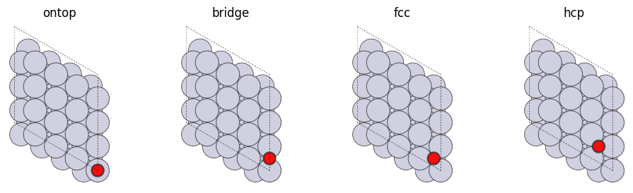
As we can see above, each adsorption site is as follows
ontop: on one atombridge: between two atomsfcc: between three atoms with no atoms in the second layerhcp: between three atoms, directly above the atom in the second layer
The adsorption site of a molecule on a surface structure is non-trivial, depending on the slab and molecular system. It is necessary to find the location where the adsorption energy is minimium (minimum energy of the adsorbed structure).
[18]:
E_slab_mol_ontop = get_opt_energy(slab_mol_ontop, fmax=1e-3)
E_slab_mol_bridge = get_opt_energy(slab_mol_bridge, fmax=1e-3)
E_slab_mol_fcc = get_opt_energy(slab_mol_fcc, fmax=1e-3)
E_slab_mol_hcp = get_opt_energy(slab_mol_hcp, fmax=1e-3)
Step Time Energy fmax
LBFGS: 0 05:01:09 -317.842408 2.898524
LBFGS: 1 05:01:09 -317.970382 3.594473
LBFGS: 2 05:01:09 -318.191282 1.677129
/tmp/ipykernel_3433/1344539460.py:7: FutureWarning: Please use atoms.calc = calc
atoms.set_calculator(calculator)
LBFGS: 3 05:01:09 -318.281448 0.675228
LBFGS: 4 05:01:09 -318.290984 0.402372
LBFGS: 5 05:01:09 -318.298270 0.037055
LBFGS: 6 05:01:09 -318.299179 0.060686
LBFGS: 7 05:01:09 -318.302309 0.184551
LBFGS: 8 05:01:09 -318.304047 0.160590
LBFGS: 9 05:01:09 -318.304851 0.053999
LBFGS: 10 05:01:09 -318.305001 0.024050
LBFGS: 11 05:01:09 -318.305081 0.019806
LBFGS: 12 05:01:10 -318.305105 0.025294
LBFGS: 13 05:01:10 -318.305111 0.013119
LBFGS: 14 05:01:10 -318.305159 0.004592
LBFGS: 15 05:01:10 -318.305176 0.004777
LBFGS: 16 05:01:10 -318.305135 0.009718
LBFGS: 17 05:01:10 -318.305175 0.010435
LBFGS: 18 05:01:10 -318.305210 0.005958
LBFGS: 19 05:01:10 -318.305214 0.001659
LBFGS: 20 05:01:10 -318.305143 0.002806
LBFGS: 21 05:01:10 -318.305147 0.003268
LBFGS: 22 05:01:10 -318.305220 0.002370
LBFGS: 23 05:01:10 -318.305214 0.001250
LBFGS: 24 05:01:10 -318.305179 0.001596
LBFGS: 25 05:01:11 -318.305176 0.002351
LBFGS: 26 05:01:11 -318.305144 0.002218
LBFGS: 27 05:01:11 -318.305219 0.001216
LBFGS: 28 05:01:11 -318.305215 0.000552
Step Time Energy fmax
LBFGS: 0 05:01:11 -317.298018 3.367196
LBFGS: 1 05:01:11 -317.432625 4.081287
LBFGS: 2 05:01:11 -317.699279 2.858173
LBFGS: 3 05:01:11 -317.973906 1.086518
LBFGS: 4 05:01:11 -317.996374 0.707769
LBFGS: 5 05:01:11 -318.071183 0.641063
LBFGS: 6 05:01:11 -318.081374 0.366953
LBFGS: 7 05:01:11 -318.087611 0.250201
LBFGS: 8 05:01:11 -318.107593 0.845663
LBFGS: 9 05:01:11 -318.115866 0.647180
LBFGS: 10 05:01:12 -318.121201 0.170366
LBFGS: 11 05:01:12 -318.123988 0.213779
LBFGS: 12 05:01:12 -318.127898 0.427406
LBFGS: 13 05:01:12 -318.130784 0.379354
LBFGS: 14 05:01:12 -318.132467 0.151580
LBFGS: 15 05:01:12 -318.133094 0.059628
LBFGS: 16 05:01:12 -318.133756 0.175862
LBFGS: 17 05:01:12 -318.134530 0.215524
LBFGS: 18 05:01:12 -318.135066 0.130313
LBFGS: 19 05:01:12 -318.135305 0.023242
LBFGS: 20 05:01:12 -318.135427 0.049550
LBFGS: 21 05:01:12 -318.135580 0.089026
LBFGS: 22 05:01:12 -318.135706 0.078572
LBFGS: 23 05:01:12 -318.135824 0.030660
LBFGS: 24 05:01:12 -318.135793 0.010860
LBFGS: 25 05:01:12 -318.135857 0.030221
LBFGS: 26 05:01:13 -318.135911 0.038738
LBFGS: 27 05:01:13 -318.135879 0.024980
LBFGS: 28 05:01:13 -318.135890 0.007104
LBFGS: 29 05:01:13 -318.135900 0.009158
LBFGS: 30 05:01:13 -318.135897 0.017172
LBFGS: 31 05:01:13 -318.135899 0.018328
LBFGS: 32 05:01:13 -318.135899 0.010433
LBFGS: 33 05:01:13 -318.135916 0.004518
LBFGS: 34 05:01:13 -318.135891 0.010585
LBFGS: 35 05:01:13 -318.135949 0.017736
LBFGS: 36 05:01:13 -318.135855 0.019821
LBFGS: 37 05:01:13 -318.135927 0.013268
LBFGS: 38 05:01:13 -318.135985 0.005323
LBFGS: 39 05:01:13 -318.135954 0.018906
LBFGS: 40 05:01:13 -318.135961 0.037519
LBFGS: 41 05:01:13 -318.135991 0.049869
LBFGS: 42 05:01:14 -318.136023 0.043147
LBFGS: 43 05:01:14 -318.136093 0.017429
LBFGS: 44 05:01:14 -318.136120 0.015111
LBFGS: 45 05:01:14 -318.136138 0.040347
LBFGS: 46 05:01:14 -318.136259 0.055027
LBFGS: 47 05:01:14 -318.136321 0.044535
LBFGS: 48 05:01:14 -318.134209 0.175405
LBFGS: 49 05:01:14 -318.136430 0.021860
LBFGS: 50 05:01:14 -318.136463 0.012867
LBFGS: 51 05:01:14 -318.136512 0.060926
LBFGS: 52 05:01:14 -318.136521 0.025587
LBFGS: 53 05:01:14 -318.136524 0.032892
LBFGS: 54 05:01:15 -318.136518 0.029711
LBFGS: 55 05:01:15 -318.136533 0.052500
LBFGS: 56 05:01:15 -318.136558 0.055009
LBFGS: 57 05:01:15 -318.136564 0.041614
LBFGS: 58 05:01:15 -318.136645 0.025558
LBFGS: 59 05:01:15 -318.136664 0.011149
LBFGS: 60 05:01:15 -318.136694 0.028943
LBFGS: 61 05:01:15 -318.136706 0.042383
LBFGS: 62 05:01:15 -318.136710 0.028344
LBFGS: 63 05:01:15 -318.136797 0.008639
LBFGS: 64 05:01:15 -318.136819 0.019556
LBFGS: 65 05:01:15 -318.136773 0.033059
LBFGS: 66 05:01:15 -318.136823 0.034832
LBFGS: 67 05:01:16 -318.136881 0.020040
LBFGS: 68 05:01:16 -318.136843 0.005330
LBFGS: 69 05:01:16 -318.136902 0.015483
LBFGS: 70 05:01:16 -318.136883 0.022676
LBFGS: 71 05:01:16 -318.136915 0.019674
LBFGS: 72 05:01:16 -318.136884 0.008090
LBFGS: 73 05:01:16 -318.136937 0.002205
LBFGS: 74 05:01:16 -318.136921 0.006972
LBFGS: 75 05:01:16 -318.136944 0.009053
LBFGS: 76 05:01:16 -318.136934 0.006030
LBFGS: 77 05:01:16 -318.136941 0.001094
LBFGS: 78 05:01:16 -318.136933 0.001779
LBFGS: 79 05:01:17 -318.136942 0.003125
LBFGS: 80 05:01:17 -318.136944 0.002603
LBFGS: 81 05:01:17 -318.136938 0.000913
Step Time Energy fmax
LBFGS: 0 05:01:17 -317.197130 3.303990
LBFGS: 1 05:01:17 -317.316486 4.021271
LBFGS: 2 05:01:17 -317.552021 2.731868
LBFGS: 3 05:01:17 -317.811816 1.460499
LBFGS: 4 05:01:17 -317.847270 1.047521
LBFGS: 5 05:01:17 -317.982363 1.271480
LBFGS: 6 05:01:17 -318.026900 1.048226
LBFGS: 7 05:01:17 -318.057192 0.314735
LBFGS: 8 05:01:18 -318.064142 0.309280
LBFGS: 9 05:01:18 -318.086642 0.740661
LBFGS: 10 05:01:18 -318.096534 0.474637
LBFGS: 11 05:01:18 -318.100364 0.116436
LBFGS: 12 05:01:18 -318.103292 0.220766
LBFGS: 13 05:01:18 -318.106737 0.353436
LBFGS: 14 05:01:18 -318.109138 0.265440
LBFGS: 15 05:01:18 -318.110216 0.078129
LBFGS: 16 05:01:18 -318.110673 0.067056
LBFGS: 17 05:01:18 -318.111208 0.155902
LBFGS: 18 05:01:18 -318.111794 0.161744
LBFGS: 19 05:01:18 -318.112151 0.078354
LBFGS: 20 05:01:19 -318.112297 0.018218
LBFGS: 21 05:01:19 -318.112343 0.045253
LBFGS: 22 05:01:19 -318.112436 0.065510
LBFGS: 23 05:01:19 -318.112558 0.047467
LBFGS: 24 05:01:19 -318.112595 0.012059
LBFGS: 25 05:01:19 -318.112616 0.014105
LBFGS: 26 05:01:19 -318.112630 0.031005
LBFGS: 27 05:01:19 -318.112652 0.031259
LBFGS: 28 05:01:19 -318.112681 0.014552
LBFGS: 29 05:01:19 -318.112650 0.002562
LBFGS: 30 05:01:19 -318.112651 0.004874
LBFGS: 31 05:01:19 -318.112656 0.007728
LBFGS: 32 05:01:19 -318.112677 0.005742
LBFGS: 33 05:01:20 -318.112668 0.001651
LBFGS: 34 05:01:20 -318.112664 0.000739
Step Time Energy fmax
LBFGS: 0 05:01:20 -317.202676 3.329409
LBFGS: 1 05:01:20 -317.323988 4.036102
LBFGS: 2 05:01:20 -317.562339 2.758290
LBFGS: 3 05:01:20 -317.827578 1.460115
LBFGS: 4 05:01:20 -317.863367 1.048154
LBFGS: 5 05:01:20 -317.998344 1.243057
LBFGS: 6 05:01:20 -318.041644 1.015544
LBFGS: 7 05:01:20 -318.070363 0.316262
LBFGS: 8 05:01:20 -318.077359 0.315765
LBFGS: 9 05:01:20 -318.102029 0.707727
LBFGS: 10 05:01:20 -318.111213 0.437634
LBFGS: 11 05:01:20 -318.115049 0.176868
LBFGS: 12 05:01:21 -318.117735 0.215533
LBFGS: 13 05:01:21 -318.121458 0.348068
LBFGS: 14 05:01:21 -318.124152 0.271505
LBFGS: 15 05:01:21 -318.125450 0.083579
LBFGS: 16 05:01:21 -318.125985 0.055497
LBFGS: 17 05:01:21 -318.126532 0.138587
LBFGS: 18 05:01:21 -318.127129 0.141324
LBFGS: 19 05:01:21 -318.127410 0.065595
LBFGS: 20 05:01:21 -318.127459 0.015101
LBFGS: 21 05:01:21 -318.127602 0.042058
LBFGS: 22 05:01:21 -318.127698 0.063686
LBFGS: 23 05:01:21 -318.127806 0.049576
LBFGS: 24 05:01:22 -318.127834 0.014832
LBFGS: 25 05:01:22 -318.127799 0.011298
LBFGS: 26 05:01:22 -318.127835 0.025439
LBFGS: 27 05:01:22 -318.127860 0.025955
LBFGS: 28 05:01:22 -318.127912 0.012118
LBFGS: 29 05:01:22 -318.127881 0.001567
LBFGS: 30 05:01:22 -318.127888 0.003975
LBFGS: 31 05:01:22 -318.127853 0.006622
LBFGS: 32 05:01:22 -318.127849 0.005111
LBFGS: 33 05:01:22 -318.127903 0.001587
LBFGS: 34 05:01:22 -318.127830 0.000604
[19]:
import pandas as pd
series = pd.Series({
"ontop": E_slab_mol_ontop,
"bridge": E_slab_mol_bridge,
"fcc": E_slab_mol_fcc,
"hcp": E_slab_mol_hcp,
})
E_adsorp_series = series - (E_slab + E_mol)
E_adsorp_series.plot(style="o-", xlabel="Adsorption site", ylabel="Energy [eV]", title="Adsorption energy for each adsorption site")
plt.show()
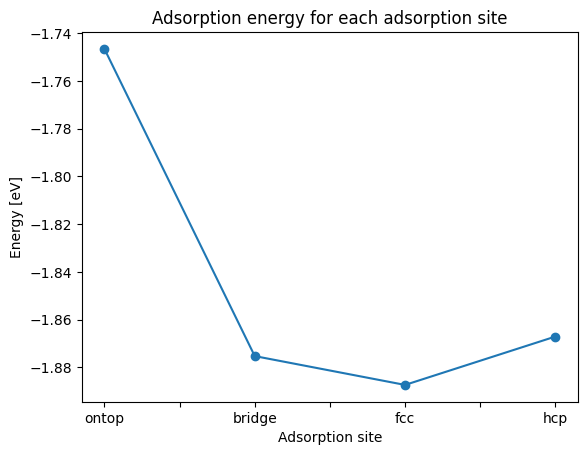
We see that the energy of the adsorption structure differs depending on the adsorption site. In this calculation, the ontop site is the most stable and has the smallest adsorption energy.
[20]:
view_ngl([slab_mol_ontop, slab_mol_bridge, slab_mol_fcc, slab_mol_hcp])
[20]:
FixAtoms constrains
All atomic coordinates were relaxed in the above calculation. But when using DFT to obtain adsorption structures, the atomic coordinates of the lower layer of slab may be fixed during structural optimization to increase the stability of the structure.
Let’s try this method by using the ASE constraint FixAtoms, we can fix the atomic coordinates at a given index.
[21]:
%%time
slab_mol_fixed = hcp0001("Co", a=a, c=c, size=(4, 4, 4), vacuum=40.0, periodic=True, orthogonal=orthogonal)
mol2 = molecule("CO")
add_adsorbate(slab_mol_fixed, mol2, 3.0, "bridge")
view_ngl(slab_mol_fixed)
CPU times: user 34.8 ms, sys: 8.03 ms, total: 42.8 ms
Wall time: 37.6 ms
[21]:
The threshold of the z coordinate is used to specify the atoms in the bottom two layers.
You can see the z coordinate from the above visualization by hovering the cursor over it, but this time, let’s visualize and check the z-axis distribution as follows.
[22]:
import pandas as pd
atoms = slab_mol_fixed
df = pd.DataFrame({
"x": atoms.positions[:, 0],
"y": atoms.positions[:, 1],
"z": atoms.positions[:, 2],
"symbol": atoms.symbols,
})
df
[22]:
| x | y | z | symbol | |
|---|---|---|---|---|
| 0 | -4.626848e-17 | 1.443662 | 40.00000 | Co |
| 1 | 2.500496e+00 | 1.443662 | 40.00000 | Co |
| 2 | 5.000993e+00 | 1.443662 | 40.00000 | Co |
| 3 | 7.501489e+00 | 1.443662 | 40.00000 | Co |
| 4 | 1.250248e+00 | 3.609156 | 40.00000 | Co |
| ... | ... | ... | ... | ... |
| 61 | 6.251241e+00 | 6.496480 | 46.03421 | Co |
| 62 | 8.751738e+00 | 6.496480 | 46.03421 | Co |
| 63 | 1.125223e+01 | 6.496480 | 46.03421 | Co |
| 64 | 1.250248e+00 | 0.000000 | 49.03421 | O |
| 65 | 1.250248e+00 | 0.000000 | 47.88387 | C |
66 rows × 4 columns
[23]:
import plotly.express as px
coord = "z"
df_sorted = df.sort_values(coord).reset_index().rename({"index": "atom_index"}, axis=1)
fig = px.scatter(df_sorted, x=df_sorted.index, y=coord, color="symbol", hover_data=["x", "y", "z", "atom_index"])
fig.show()
The boundary between the second and third layers was found to be between 42.03 - 44.07.
The FixAtoms can be used by either setting an index of atoms to fix in the indices or setting an array of bool to fix or not to fix each atom in the mask.
We will use mask in this example.
[24]:
from ase.constraints import FixAtoms
thresh = 43.0
constraint = FixAtoms(mask=slab_mol_fixed.positions[:, 2] < thresh)
constraint
[24]:
FixAtoms(indices=[0, 1, 2, 3, 4, 5, 6, 7, 8, 9, 10, 11, 12, 13, 14, 15, 16, 17, 18, 19, 20, 21, 22, 23, 24, 25, 26, 27, 28, 29, 30, 31])
The created constraint can be set with the atoms.set_constraint method.
[25]:
slab_mol_fixed.set_constraint(constraint)
Visualize and check that the intended location is fixed.
[26]:
v = view_ngl(slab_mol_fixed)
v.show_fix_atoms_constraint()
v
[26]:
[27]:
E_slab_mol_fixed = get_opt_energy(slab_mol_fixed, fmax=1e-3)
Step Time Energy fmax
LBFGS: 0 05:01:23 -317.298046 3.367193
LBFGS: 1 05:01:23 -317.370433 4.084981
/tmp/ipykernel_3433/1344539460.py:7: FutureWarning:
Please use atoms.calc = calc
LBFGS: 2 05:01:23 -317.549330 2.528261
LBFGS: 3 05:01:24 -317.833422 2.157216
LBFGS: 4 05:01:24 -317.865740 0.838110
LBFGS: 5 05:01:24 -317.899339 0.966453
LBFGS: 6 05:01:24 -317.922718 1.125139
LBFGS: 7 05:01:24 -317.936185 0.675126
LBFGS: 8 05:01:24 -317.943700 0.249672
LBFGS: 9 05:01:24 -317.948898 0.451393
LBFGS: 10 05:01:24 -317.956971 0.705947
LBFGS: 11 05:01:24 -317.963627 0.549626
LBFGS: 12 05:01:24 -317.966968 0.200157
LBFGS: 13 05:01:24 -317.968894 0.193649
LBFGS: 14 05:01:24 -317.971012 0.367471
LBFGS: 15 05:01:24 -317.973073 0.366748
LBFGS: 16 05:01:24 -317.974495 0.185133
LBFGS: 17 05:01:25 -317.975121 0.052330
LBFGS: 18 05:01:25 -317.975567 0.124829
LBFGS: 19 05:01:25 -317.976069 0.179915
LBFGS: 20 05:01:25 -317.976485 0.130129
LBFGS: 21 05:01:25 -317.976679 0.036992
LBFGS: 22 05:01:25 -317.976742 0.032473
LBFGS: 23 05:01:25 -317.976841 0.067961
LBFGS: 24 05:01:25 -317.976913 0.067908
LBFGS: 25 05:01:25 -317.976948 0.032542
LBFGS: 26 05:01:25 -317.976991 0.006594
LBFGS: 27 05:01:25 -317.977004 0.018813
LBFGS: 28 05:01:26 -317.977011 0.032035
LBFGS: 29 05:01:26 -317.977034 0.029605
LBFGS: 30 05:01:26 -317.977043 0.013607
LBFGS: 31 05:01:26 -317.977053 0.005401
LBFGS: 32 05:01:26 -317.977055 0.012157
LBFGS: 33 05:01:26 -317.977064 0.017967
LBFGS: 34 05:01:26 -317.977071 0.015757
LBFGS: 35 05:01:26 -317.977069 0.007217
LBFGS: 36 05:01:26 -317.977020 0.007363
LBFGS: 37 05:01:26 -317.977075 0.017915
LBFGS: 38 05:01:26 -317.977102 0.029666
LBFGS: 39 05:01:26 -317.977073 0.035775
LBFGS: 40 05:01:27 -317.977122 0.027862
LBFGS: 41 05:01:27 -317.977149 0.010232
LBFGS: 42 05:01:27 -317.977187 0.019037
LBFGS: 43 05:01:27 -317.977211 0.042417
LBFGS: 44 05:01:27 -317.977241 0.055570
LBFGS: 45 05:01:27 -317.977295 0.044879
LBFGS: 46 05:01:27 -317.977276 0.015693
LBFGS: 47 05:01:27 -317.977347 0.011269
LBFGS: 48 05:01:27 -317.977329 0.028472
LBFGS: 49 05:01:27 -317.977419 0.037660
LBFGS: 50 05:01:27 -317.976700 0.042962
LBFGS: 51 05:01:28 -317.977447 0.028700
LBFGS: 52 05:01:28 -317.977466 0.020285
LBFGS: 53 05:01:28 -317.975169 0.217418
LBFGS: 54 05:01:28 -317.977530 0.010444
LBFGS: 55 05:01:28 -317.977554 0.010728
LBFGS: 56 05:01:28 -317.976147 0.167147
LBFGS: 57 05:01:28 -317.977605 0.015344
LBFGS: 58 05:01:28 -317.977641 0.018246
LBFGS: 59 05:01:28 -317.975360 0.152353
LBFGS: 60 05:01:28 -317.977710 0.019435
LBFGS: 61 05:01:29 -317.977729 0.020207
LBFGS: 62 05:01:29 -317.977740 0.019599
LBFGS: 63 05:01:29 -317.977792 0.015333
LBFGS: 64 05:01:29 -317.977923 0.026060
LBFGS: 65 05:01:29 -317.977937 0.029808
LBFGS: 66 05:01:29 -317.978010 0.027831
LBFGS: 67 05:01:29 -317.978059 0.012066
LBFGS: 68 05:01:29 -317.978089 0.013912
LBFGS: 69 05:01:29 -317.978113 0.022272
LBFGS: 70 05:01:29 -317.978131 0.025347
LBFGS: 71 05:01:30 -317.978144 0.016545
LBFGS: 72 05:01:30 -317.978148 0.002875
LBFGS: 73 05:01:30 -317.978164 0.004765
LBFGS: 74 05:01:30 -317.978164 0.007394
LBFGS: 75 05:01:30 -317.978161 0.006962
LBFGS: 76 05:01:30 -317.978175 0.003307
LBFGS: 77 05:01:30 -317.978126 0.001155
LBFGS: 78 05:01:30 -317.978161 0.002111
LBFGS: 79 05:01:30 -317.978178 0.003076
LBFGS: 80 05:01:31 -317.978163 0.002670
LBFGS: 81 05:01:31 -317.978175 0.001194
LBFGS: 82 05:01:31 -317.978169 0.000279
[28]:
E_adsorp = E_slab_mol_fixed - (E_slab + E_mol)
print(f"E_adsorp {E_adsorp}, E_slab_mol {E_slab_mol_fixed}, E_slab {E_slab}, E_mol {E_mol}")
E_adsorp -1.3960754815630594, E_slab_mol -317.9781686732514, E_slab -305.13616061153743, E_mol -11.445932580150906
When the lower layer is fixed, an adsorption energy of -1.19 eV was obtained.
CO on Pd
Let’s calculate CO adsorption on Pd in the same manner.
[29]:
import numpy as np
bulk_atoms = bulk("Pd", cubic=True)
np.mean(np.diag(bulk_atoms.cell))
[29]:
3.89
[30]:
bulk_atoms.calc = calculator
E_bulk = get_opt_energy(bulk_atoms, fmax=1e-4, opt_mode="scale")
a_pd = np.mean(np.diag(bulk_atoms.cell))
a_pd
Step Time Energy fmax
LBFGS: 0 05:01:31 -14.904795 4.593262
LBFGS: 1 05:01:31 -14.805114 7.050895
/tmp/ipykernel_3433/1344539460.py:7: FutureWarning:
Please use atoms.calc = calc
/tmp/ipykernel_3433/1344539460.py:9: FutureWarning:
Import StrainFilter from ase.filters
LBFGS: 2 05:01:31 -14.954530 0.571581
LBFGS: 3 05:01:31 -14.955401 0.069699
LBFGS: 4 05:01:31 -14.955413 0.000910
LBFGS: 5 05:01:31 -14.955418 0.000067
[30]:
3.941105705982878
[31]:
from ase.build import fcc111, molecule, add_adsorbate
slab = fcc111("Pd", a=a_pd, size=(4, 4, 4), vacuum=40.0, periodic=True)
slab.calc = calculator
E_slab = get_opt_energy(slab, fmax=1e-4, opt_mode="normal")
Step Time Energy fmax
LBFGS: 0 05:01:31 -221.469662 0.154306
LBFGS: 1 05:01:31 -221.479485 0.123494
/tmp/ipykernel_3433/1344539460.py:7: FutureWarning:
Please use atoms.calc = calc
LBFGS: 2 05:01:32 -221.497979 0.037257
LBFGS: 3 05:01:32 -221.498799 0.037970
LBFGS: 4 05:01:32 -221.502356 0.031879
LBFGS: 5 05:01:32 -221.504820 0.024933
LBFGS: 6 05:01:32 -221.505937 0.009735
LBFGS: 7 05:01:32 -221.506049 0.001465
LBFGS: 8 05:01:32 -221.505994 0.000064
[32]:
mol = molecule("CO")
mol.calc = calculator
E_mol = get_opt_energy(mol, fmax=1e-4)
Step Time Energy fmax
LBFGS: 0 05:01:32 -11.443040 0.797118
LBFGS: 1 05:01:32 -11.431572 1.878737
LBFGS: 2 05:01:32 -11.445922 0.046010
/tmp/ipykernel_3433/1344539460.py:7: FutureWarning:
Please use atoms.calc = calc
LBFGS: 3 05:01:32 -11.445935 0.002584
LBFGS: 4 05:01:32 -11.445933 0.000005
[33]:
%%time
slab_mol = fcc111("Pd", a=a_pd, size=(4, 4, 4), vacuum=40.0)
slab_mol.pbc = True
mol2 = molecule("CO")
add_adsorbate(slab_mol, mol2, 3.0, "ontop")
E_slab_mol = get_opt_energy(slab_mol, fmax=1e-3)
Step Time Energy fmax
LBFGS: 0 05:01:32 -234.320127 0.953715
LBFGS: 1 05:01:32 -234.323178 1.770322
/tmp/ipykernel_3433/1344539460.py:7: FutureWarning:
Please use atoms.calc = calc
LBFGS: 2 05:01:33 -234.347470 0.538091
LBFGS: 3 05:01:33 -234.365402 0.473518
LBFGS: 4 05:01:33 -234.371691 0.360437
LBFGS: 5 05:01:33 -234.374841 0.099046
LBFGS: 6 05:01:33 -234.378273 0.241564
LBFGS: 7 05:01:33 -234.382273 0.348405
LBFGS: 8 05:01:33 -234.384511 0.231276
LBFGS: 9 05:01:33 -234.385570 0.061829
LBFGS: 10 05:01:33 -234.386380 0.145362
LBFGS: 11 05:01:33 -234.387563 0.253167
LBFGS: 12 05:01:33 -234.388719 0.241592
LBFGS: 13 05:01:34 -234.389416 0.121320
LBFGS: 14 05:01:34 -234.389756 0.048352
LBFGS: 15 05:01:34 -234.390049 0.111616
LBFGS: 16 05:01:34 -234.390455 0.144710
LBFGS: 17 05:01:34 -234.390915 0.120400
LBFGS: 18 05:01:34 -234.391242 0.046067
LBFGS: 19 05:01:34 -234.391444 0.028925
LBFGS: 20 05:01:34 -234.391634 0.079809
LBFGS: 21 05:01:34 -234.391843 0.091986
LBFGS: 22 05:01:34 -234.391979 0.054356
LBFGS: 23 05:01:34 -234.392042 0.017186
LBFGS: 24 05:01:34 -234.392074 0.017494
LBFGS: 25 05:01:34 -234.392081 0.022621
LBFGS: 26 05:01:35 -234.392087 0.014591
LBFGS: 27 05:01:35 -234.392116 0.007934
LBFGS: 28 05:01:35 -234.392105 0.009305
LBFGS: 29 05:01:35 -234.392121 0.005786
LBFGS: 30 05:01:35 -234.392116 0.005674
LBFGS: 31 05:01:35 -234.392125 0.004706
LBFGS: 32 05:01:35 -234.392135 0.004091
LBFGS: 33 05:01:35 -234.392113 0.003857
LBFGS: 34 05:01:35 -234.392124 0.003134
LBFGS: 35 05:01:35 -234.392117 0.004607
LBFGS: 36 05:01:35 -234.392149 0.004598
LBFGS: 37 05:01:36 -234.392152 0.002170
LBFGS: 38 05:01:36 -234.392129 0.000932
CPU times: user 221 ms, sys: 18.1 ms, total: 239 ms
Wall time: 3.27 s
[34]:
E_adsorp = E_slab_mol - (E_slab + E_mol)
print(f"E_adsorp {E_adsorp}, E_slab_mol {E_slab_mol}, E_slab {E_slab}, E_mol {E_mol}")
E_adsorp -1.4402008748295714, E_slab_mol -234.39212860995127, E_slab -221.50599434099485, E_mol -11.445933394126861
[35]:
from pfcc_extras.visualize.view import view_ngl
view_ngl(slab_mol)
[35]:
In this way, adsorption energies can be calculated for various surface and molecular combinations. This is an essential process in the search for efficient catalysts, which will be discussed in chapter 5.
Coverage ratio
In the example discussed in this tutorial, only one molecule is adsorbed on a surface. In reality, there are cases where many molecules react with the surface at the same time, where multiple molecules are adsorbed at the same time, or where the surface is almost completely covered with adsorbed molecules.
In this case, we are interested in the adsorption energy of a single molecule adsorbed on a slab where multiple molecules are already adsorbed.
The analysis of the coverage ratio dependency of the adsorption energy of CO molecules on the Pd surface is reported in the following literature
Adsorption to multiple locations
Another application topic not covered here is adsorption to more than one location. When molecules are large and complex, there are some cases that become stable by adsorbing to multiple locations on the surface.