Optimization algorithm
前節まででは様々な事例に対して、 構造最適化を適用してみました。 本節では、構造最適化の際に適用を行った局所最適化アルゴリズムについて学んでいきます。
アルゴリズムの種類
局所最適化アルゴリズムとして、ASEではMolecular Dynamics (MD)に似た振る舞いで最適化を行う FIRE や、2次関数近似をおこなって最適化を行う BFGS, LBFGS, BFGSLineSearch=QuasiNewton, LBFGSLineSearch法などが提供されています。
アルゴリズム |
グループ |
特徴 |
|---|---|---|
MDMin |
MD-like |
MDを行うが、運動量とForceの内積が負になると運動量を0にリセットする |
FIRE |
MD-like |
MDを行うが、様々な追加の工夫を入れて高速かつ頑健にしたもの |
BFGS |
準Newton法 |
最適化のトラジェクトリからヘシアンを近似し、近似ヘシアンを用いてNewton法のアルゴリズムを実行 |
LBFGS |
準Newton法 |
BFGS法を高速・低メモリで動くようにしたもの |
BFGSLineSearch |
準Newton法 |
BFGSで最適化のステップの方向を決定し、ステップの大きさはLineSearchで決定 |
LBFGSLineSearch |
準Newton法 |
LBFGSで最適化のステップの方向を決定し、ステップの大きさはLineSearchで決定 |
MDMinはハイパーパラメーター依存性が大きく、構造最適化に失敗することも多いためベンチマークから除外し、他のOptimizerを見ていきます。
FIRE
FIREでは基本的にMDを行いますが、高速に収束するように様々な工夫が加えられています。
ニュートン法
ニュートン法ではヘシアンと勾配を用いて次のステップを決定します。ニュートン法は二次収束する手法であり、ポテンシャルが二次関数に近い時(極小点に近い時)真の解に二乗の速度で近づいていき非常に高速です。 ヘシアンを \(H\)、勾配を \(\vec{g}\) として、次の最適化ステップ \(\vec{p}\) を以下の式で表現します。
\(\vec{p} = - H^{-1} \vec{g}\)
仮にポテンシャルが厳密に二次関数であれば1ステップで極小値に収束します。
準ニュートン法
BFGS
LBFGS
LineSearch
ベンチマーク
[1]:
import os
from time import perf_counter
from typing import Optional, Type

import matplotlib.pyplot as plt
import pandas as pd
from ase import Atoms
from ase.build import bulk, molecule
from ase.calculators.calculator import Calculator
from ase.io import Trajectory
from ase.optimize import BFGS, FIRE, LBFGS, BFGSLineSearch, LBFGSLineSearch, MDMin
from ase.optimize.optimize import Optimizer
from tqdm.auto import tqdm

import pfp_api_client
from pfcc_extras.structure.ase_rdkit_converter import atoms_to_smiles, smiles_to_atoms
from pfcc_extras.visualize.view import view_ngl
from pfp_api_client.pfp.calculators.ase_calculator import ASECalculator
from pfp_api_client.pfp.estimator import Estimator, EstimatorCalcMode
[2]:
calc = ASECalculator(Estimator(calc_mode=EstimatorCalcMode.PBE, model_version="v8.0.0"))
calc_mol = ASECalculator(Estimator(calc_mode=EstimatorCalcMode.WB97XD, model_version="v8.0.0"))
print(f"pfp_api_client: {pfp_api_client.__version__}")
print(calc.estimator.model_version)
pfp_api_client: 1.23.1
v8.0.0
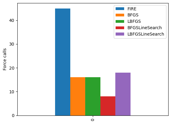
Force計算回数の比較
molecule("CH3CHO") で得られる構造は厳密な安定構造ではありませんが、かなり良い構造をしています。[3]:
def get_force_calls(opt: Optimizer) -> int:
    """Obtrain number of force calculations"""
    if isinstance(opt, (BFGSLineSearch, LBFGSLineSearch)):
        return opt.force_calls
    else:
        return opt.nsteps
[4]:
os.makedirs("output", exist_ok=True)
[5]:
atoms_0 = bulk("Pt") * (4, 4, 4)
atoms_0.rattle(stdev=0.1)
[6]:
view_ngl(atoms_0)
[6]:
[7]:
force_calls = {}
for opt_class in tqdm([FIRE, BFGS, LBFGS, BFGSLineSearch, LBFGSLineSearch]):
    atoms = atoms_0.copy()
    atoms.calc = calc
    name = opt_class.__name__
    with opt_class(atoms, trajectory=f"output/{name}_ch3cho.traj", logfile=None) as opt:
        opt.run(fmax=0.05)
        force_calls[name] = [get_force_calls(opt)]
[8]:
df = pd.DataFrame.from_dict(force_calls)
df.plot.bar()
plt.ylabel("Force calls")
plt.show()
1ステップあたりの速度比較
次に同じそれぞれの最適化手法の1stepあたりの速度を比較してみます。
[9]:
from ase.build import bulk

atoms = bulk("Fe") * (10, 5, 3)
atoms.rattle(stdev=0.2)
atoms.calc = calc

view_ngl(atoms)
[9]:
[10]:
def opt_benchmark(atoms: Atoms, calculator: Calculator, opt_class, logfile: Optional[str] = "-", steps: int = 10) -> float:
    _atoms = atoms.copy()
    _atoms.calc = calculator
    with opt_class(_atoms, logfile=logfile) as opt:
        start_time = perf_counter()
        opt.run(steps=steps)
        end_time = perf_counter()
        duration = end_time - start_time
        duration_per_force_calls = duration / get_force_calls(opt)
    return duration_per_force_calls
[11]:
result_dict = {
    "n_atoms": [],
    "FIRE": [],
    "BFGS": [],
    "LBFGS": [],
    "BFGSLineSearch": [],
    "LBFGSLineSearch": [],
}


for i in range(1, 10):
    atoms = bulk("Fe") * (10, 10, i)
    atoms.rattle(stdev=0.2)
    n_atoms = atoms.get_global_number_of_atoms()
    result_dict["n_atoms"].append(n_atoms)
    print(f"----- n_atoms {n_atoms} -----")
    for opt_class in [FIRE, BFGS, LBFGS, BFGSLineSearch, LBFGSLineSearch]:
        name = opt_class.__name__
        print(f"Running {name}...")
        duration = opt_benchmark(atoms, calc, opt_class=opt_class, logfile=None, steps=10)
        print(f"Done in {duration:.2f} sec.")
        result_dict[name].append(duration)
----- n_atoms 100 -----
Running FIRE...
Done in 0.10 sec.
Running BFGS...
Done in 0.10 sec.
Running LBFGS...
Done in 0.09 sec.
Running BFGSLineSearch...
Done in 0.08 sec.
Running LBFGSLineSearch...
Done in 0.08 sec.
----- n_atoms 200 -----
Running FIRE...
Done in 0.09 sec.
Running BFGS...
Done in 0.15 sec.
Running LBFGS...
Done in 0.09 sec.
Running BFGSLineSearch...
Done in 0.11 sec.
Running LBFGSLineSearch...
Done in 0.09 sec.
----- n_atoms 300 -----
Running FIRE...
Done in 0.13 sec.
Running BFGS...
Done in 0.29 sec.
Running LBFGS...
Done in 0.15 sec.
Running BFGSLineSearch...
Done in 0.18 sec.
Running LBFGSLineSearch...
Done in 0.10 sec.
----- n_atoms 400 -----
Running FIRE...
Done in 0.08 sec.
Running BFGS...
Done in 0.42 sec.
Running LBFGS...
Done in 0.10 sec.
Running BFGSLineSearch...
Done in 0.19 sec.
Running LBFGSLineSearch...
Done in 0.08 sec.
----- n_atoms 500 -----
Running FIRE...
Done in 0.10 sec.
Running BFGS...
Done in 0.73 sec.
Running LBFGS...
Done in 0.09 sec.
Running BFGSLineSearch...
Done in 0.26 sec.
Running LBFGSLineSearch...
Done in 0.10 sec.
----- n_atoms 600 -----
Running FIRE...
Done in 0.10 sec.
Running BFGS...
Done in 1.28 sec.
Running LBFGS...
Done in 0.10 sec.
Running BFGSLineSearch...
Done in 0.40 sec.
Running LBFGSLineSearch...
Done in 0.11 sec.
----- n_atoms 700 -----
Running FIRE...
Done in 0.14 sec.
Running BFGS...
Done in 2.03 sec.
Running LBFGS...
Done in 0.11 sec.
Running BFGSLineSearch...
Done in 0.61 sec.
Running LBFGSLineSearch...
Done in 0.12 sec.
----- n_atoms 800 -----
Running FIRE...
Done in 0.14 sec.
Running BFGS...
Done in 3.07 sec.
Running LBFGS...
Done in 0.15 sec.
Running BFGSLineSearch...
Done in 0.84 sec.
Running LBFGSLineSearch...
Done in 0.14 sec.
----- n_atoms 900 -----
Running FIRE...
Done in 0.13 sec.
Running BFGS...
Done in 4.62 sec.
Running LBFGS...
Done in 0.12 sec.
Running BFGSLineSearch...
Done in 1.06 sec.
Running LBFGSLineSearch...
Done in 0.13 sec.
[12]:
import matplotlib.pyplot as plt
import pandas as pd

fig, axes = plt.subplots(1, 2, tight_layout=True, figsize=(10, 4))
df = pd.DataFrame(result_dict)
df = df.set_index("n_atoms")
df.plot(ax=axes[0])
axes[0].set_title("Speed for various opt algorithms")
df[["LBFGS", "FIRE", "LBFGSLineSearch"]].plot(ax=axes[1])
axes[1].set_title("Speed for various opt algorithms ($O(N)$ methods only)")
for ax in axes:
    ax.set_ylabel("sec / step")
fig.savefig("output/opt_benchmark.png")
plt.show(fig)
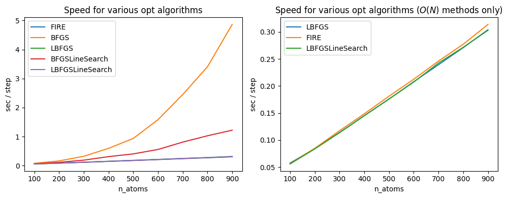
BFGSやBFGSLineSearchでは原子数が多くなるにつれて1ステップあたりの計算時間が長くなってしまっています。
最適化アルゴリズムの使い分け
LBFGSやBFGSがうまくいかない例
次の例を見てみましょう。 この例ではとても単純なポテンシャルである Lennard-Jones (LJ) potentialを用いて、その安定点から離れたところを初期値として構造最適化を行っています。
LJ potential は次式で表される形をしており、以下のような形をしています。
[13]:
from ase.calculators.lj import LennardJones
import numpy as np


calc_lj = LennardJones()

dists = np.linspace(1.0, 4.0, 500)


E_pot_list = []
for d in dists:
    atoms = Atoms("Ar2", [[0, 0, 0], [d, 0, 0]])
    atoms.calc = calc_lj
    E_pot = atoms.get_potential_energy()
    E_pot_list.append(E_pot)

plt.plot(dists, E_pot_list)
plt.title("Lennard Jones Potential")
plt.ylabel("eV")
plt.xlabel("Distance [A]")
plt.show()
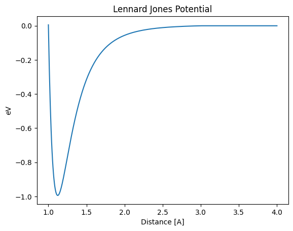
この単純なPotential の形でDistanceを安定点である1.12A から離れたところからスタートし構造最適化をしてみましょう。
[14]:
def lennard_jones_trajectory(opt_class: Type[Optimizer], d0: float):
    name = opt_class.__name__
    trajectory_path = f"output/Ar_{name}.traj"

    atoms = Atoms("Ar2", [[0, 0, 0], [d0, 0, 0]])
    atoms.calc = calc_lj

    opt = opt_class(atoms, trajectory=trajectory_path)
    opt.run()

    distance_list = []
    energy_list = []
    for atoms in Trajectory(trajectory_path):
        energy_list.append(atoms.get_potential_energy())
        distance_list.append(atoms.get_distance(0, 1))

    print("Distance in opt trajectory: ", distance_list)

    plt.plot(dists, E_pot_list)
    plt.plot(distance_list, energy_list, marker="x")
    plt.title(f"Lennard Jones Potential: {name} opt")
    plt.ylim(-1.0, 0)
    plt.ylabel("eV")
    plt.xlabel("Distance [A]")
    plt.show()
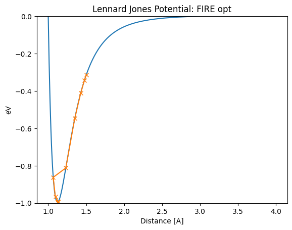
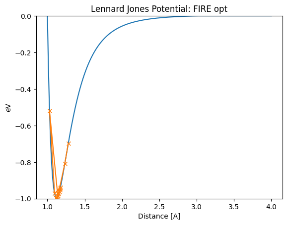
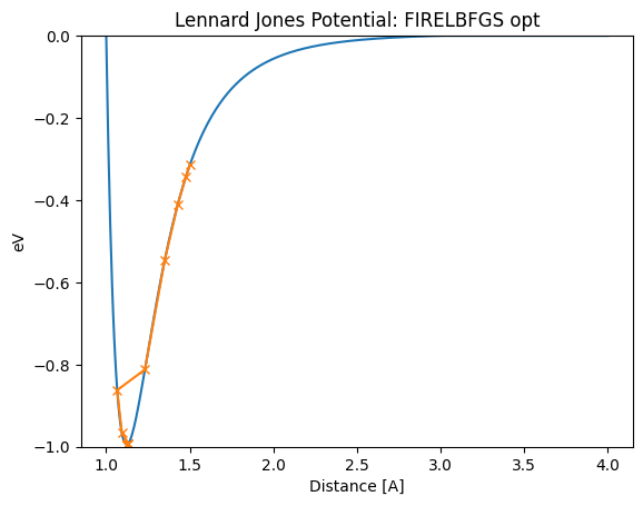
まずはFIREを行った場合です。安定して最適値1.12A にたどり着くことが出来ています。
[15]:
lennard_jones_trajectory(FIRE, 1.5)
      Step     Time          Energy          fmax
FIRE:    0 04:30:07       -0.314857        1.158029
FIRE:    1 04:30:07       -0.342894        1.264380
FIRE:    2 04:30:07       -0.410024        1.512419
FIRE:    3 04:30:07       -0.546744        1.968308
FIRE:    4 04:30:07       -0.812180        2.383891
FIRE:    5 04:30:07       -0.862167        5.585844
FIRE:    6 04:30:07       -0.966377        2.149190
FIRE:    7 04:30:07       -0.991817        0.522302
FIRE:    8 04:30:07       -0.992148        0.491275
FIRE:    9 04:30:07       -0.992732        0.429940
FIRE:   10 04:30:07       -0.993427        0.339973
FIRE:   11 04:30:07       -0.994057        0.224455
FIRE:   12 04:30:07       -0.994451        0.088426
FIRE:   13 04:30:07       -0.994489        0.060610
FIRE:   14 04:30:07       -0.994490        0.059506
FIRE:   15 04:30:07       -0.994492        0.057320
FIRE:   16 04:30:07       -0.994495        0.054094
FIRE:   17 04:30:07       -0.994499        0.049889
Distance in opt trajectory:  [1.5, 1.4768394233790767, 1.42839123774426, 1.349694678243147, 1.231631957294667, 1.0658914242047832, 1.0938206432760949, 1.132495812583008, 1.1318429355798734, 1.1305759647542164, 1.1287715691339621, 1.1265422074054834, 1.1240322773166505, 1.1214118150599879, 1.1214307556785812, 1.1214682920288386, 1.1215237409768002, 1.1215960942672192]
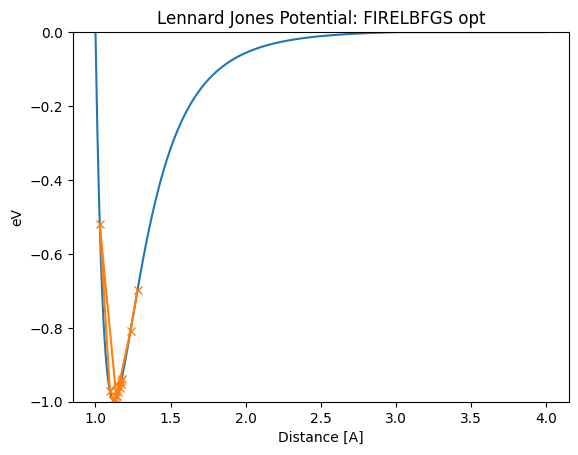
[16]:
lennard_jones_trajectory(FIRE, 1.28)
      Step     Time          Energy          fmax
FIRE:    0 04:30:08       -0.697220        2.324552
FIRE:    1 04:30:08       -0.807702        2.387400
FIRE:    2 04:30:08       -0.987241        0.821987
FIRE:    3 04:30:08       -0.520102       13.570402
FIRE:    4 04:30:08       -0.971689        1.903593
FIRE:    5 04:30:08       -0.939109        1.840004
FIRE:    6 04:30:08       -0.943288        1.793714
FIRE:    7 04:30:08       -0.951214        1.694594
FIRE:    8 04:30:08       -0.961964        1.529352
FIRE:    9 04:30:08       -0.974030        1.277952
FIRE:   10 04:30:08       -0.985244        0.914936
FIRE:   11 04:30:08       -0.992867        0.414203
FIRE:   12 04:30:08       -0.994043        0.239611
FIRE:   13 04:30:08       -0.994061        0.235001
FIRE:   14 04:30:08       -0.994095        0.225890
FIRE:   15 04:30:08       -0.994143        0.212487
FIRE:   16 04:30:08       -0.994201        0.195100
FIRE:   17 04:30:08       -0.994265        0.174121
FIRE:   18 04:30:08       -0.994330        0.150013
FIRE:   19 04:30:08       -0.994391        0.123296
FIRE:   20 04:30:08       -0.994449        0.091418
FIRE:   21 04:30:08       -0.994495        0.054286
FIRE:   22 04:30:08       -0.994519        0.012221
Distance in opt trajectory:  [1.28, 1.2335089629222111, 1.1392699328939198, 1.0285911631178963, 1.0964431714345662, 1.1738131464936081, 1.1715131413850235, 1.1669709941864936, 1.160310604717144, 1.1517385248429906, 1.1415690055780352, 1.130255815977825, 1.118424872251103, 1.1184997505580012, 1.1186480666965142, 1.1188669733107373, 1.1191522821112356, 1.1194985597723826, 1.1198992503739216, 1.1203468201911215, 1.1208857684008715, 1.121520438052656, 1.1222486280893154]
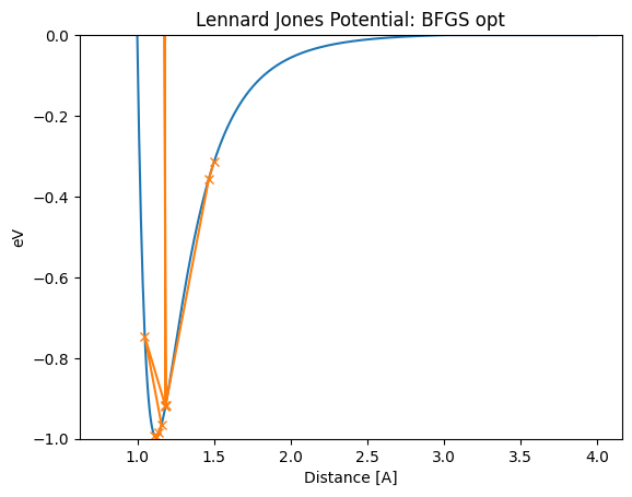
BFGS法を1.5Aから開始した場合、特定のstepではあまりにも大きくジャンプしてしまい、安定点を大きく飛び越えるような不安定な挙動になっていることがわかります。 (1.18A –> 0.78Aにジャンプしているようなところです。) このように、最適値1.12A にたどり着くまでに、この単純な例でも大きく振動しまいます。 これは2次の近似を行う手法では、関数曲面が2次関数と異なる場合に、その極小値の見積もりが大きくはずれてしまうために起こります。
[17]:
lennard_jones_trajectory(BFGS, 1.5)
      Step     Time          Energy          fmax
BFGS:    0 04:30:08       -0.314857        1.158029
BFGS:    1 04:30:08       -0.355681        1.312428
BFGS:    2 04:30:08       -0.916039        2.041011
BFGS:    3 04:30:08       55.304434      974.487533
BFGS:    4 04:30:08       -0.917740        2.028761
BFGS:    5 04:30:08       -0.919418        2.016337
BFGS:    6 04:30:08       -0.747080        8.517609
BFGS:    7 04:30:08       -0.965068        1.472894
BFGS:    8 04:30:08       -0.984660        0.939655
BFGS:    9 04:30:08       -0.992324        0.528593
BFGS:   10 04:30:08       -0.994444        0.092418
BFGS:   11 04:30:08       -0.994520        0.007274
Distance in opt trajectory:  [1.5, 1.4669134619701096, 1.1856710148074785, 0.7856710148074794, 1.1848349876531552, 1.1840057048694352, 1.0494144415981015, 1.1582431525834522, 1.1421985974452062, 1.1139254943723917, 1.1241042745909042, 1.1225894828343739]
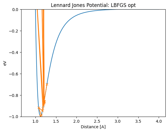
[18]:
lennard_jones_trajectory(LBFGS, 1.28)
       Step     Time          Energy          fmax
LBFGS:    0 04:30:08       -0.697220        2.324552
LBFGS:    1 04:30:08       -0.854683        2.314904
LBFGS:    2 04:30:08       33.771592      599.751912
LBFGS:    3 04:30:08       -0.858237        2.305680
LBFGS:    4 04:30:08       -0.861748        2.295944
LBFGS:    5 04:30:08       17.305333      318.491824
LBFGS:    6 04:30:08       -0.867638        2.278148
LBFGS:    7 04:30:08       -0.873395        2.258876
LBFGS:    8 04:30:08        5.604073      121.154807
LBFGS:    9 04:30:08       -0.885566        2.211348
LBFGS:   10 04:30:08       -0.897001        2.157091
LBFGS:   11 04:30:08        0.369118       30.787165
LBFGS:   12 04:30:08       -0.925197        1.970726
LBFGS:   13 04:30:08       -0.947015        1.749104
LBFGS:   14 04:30:08       -0.915603        4.009032
LBFGS:   15 04:30:08       -0.985429        0.906882
LBFGS:   16 04:30:08       -0.993163        0.377052
LBFGS:   17 04:30:08       -0.994465        0.080647
LBFGS:   18 04:30:08       -0.994520        0.005364
Distance in opt trajectory:  [1.28, 1.213584232746016, 0.813584232746016, 1.2120462614888505, 1.2105202846657441, 0.8506725019776178, 1.2079447803538972, 1.2054073889508412, 0.9079986088524912, 1.1999638317862706, 1.1947303311793407, 0.9866659932915066, 1.1811069055371053, 1.169409273526655, 1.0770879993440852, 1.1413655567592533, 1.1295077111909069, 1.1210690913427286, 1.1225559889249785]
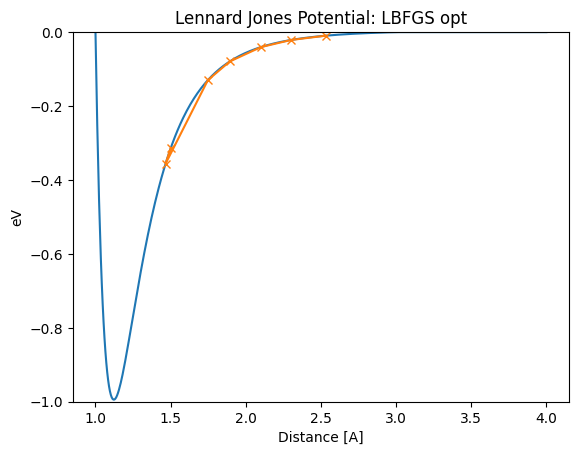
また、他にも初期値が安定点から離れたところからスタートした場合に正しく安定点にたどり着けていないケースも有ります。 これは、Hessianの初期化がうまく行かないなどの理由で起きていると考えられます。
[19]:
lennard_jones_trajectory(LBFGS, 1.50)
       Step     Time          Energy          fmax
LBFGS:    0 04:30:09       -0.314857        1.158029
LBFGS:    1 04:30:09       -0.355681        1.312428
LBFGS:    2 04:30:09       -0.129756        0.447300
LBFGS:    3 04:30:09       -0.079409        0.263016
LBFGS:    4 04:30:09       -0.040472        0.129677
LBFGS:    5 04:30:09       -0.021155        0.068924
LBFGS:    6 04:30:09       -0.009646        0.035707
Distance in opt trajectory:  [1.5, 1.4669134619701096, 1.748155909132741, 1.8935676545167726, 2.101103976550205, 2.302941039822042, 2.531922335240822]
[20]:
lennard_jones_trajectory(LBFGSLineSearch, 1.5)
                 Step     Time          Energy          fmax
LBFGSLineSearch:    0 04:30:09       -0.314857        1.158029
LBFGSLineSearch:    1 04:30:09       -0.994517        0.021446
Distance in opt trajectory:  [1.5, 1.1220880716401869]
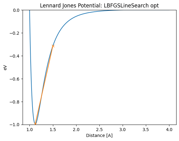
LBFGSLineSearchでは1ステップで終了しているように見えますが、内部でLineSearchを行っている部分がステップにカウントされていないため、実際の計算数はもう少し多いです。 BFGSLineSearchでは Step[FC]という表示がありますが、このFCが実際のフォース評価回数です。
[21]:
lennard_jones_trajectory(BFGSLineSearch, 1.5)
                Step[ FC]     Time          Energy          fmax
BFGSLineSearch:    0[  0] 04:30:09       -0.314857       1.1580
BFGSLineSearch:    1[  5] 04:30:09       -0.994057       0.2244
BFGSLineSearch:    2[  7] 04:30:09       -0.994520       0.0054
Distance in opt trajectory:  [1.5, 1.1265420003736115, 1.1225561293552997]
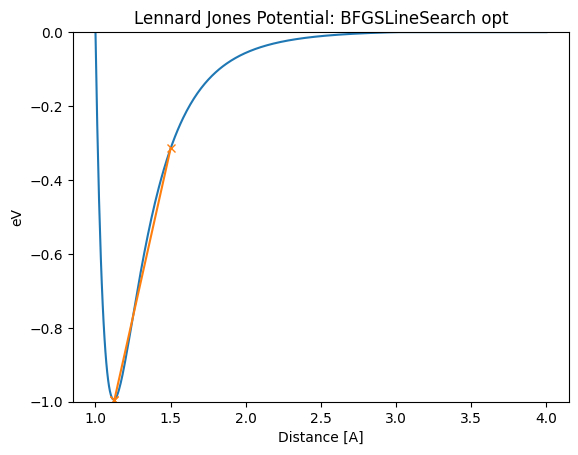
ここではBFGSやLBFGSがうまくいかない例があることを見てきました。 しかし、このような例であってもLBFGSLineSearchはうまくいっています。
FIRE: 収束までのステップ数が長い
BFGS: 原子数が多い時に計算時間がかかる。
BFGSLineSearch: 原子数が多い時に計算時間がかかる。
LBFGS: 振動したり、エネルギーが上がってしまう場合がある。
しかし、常にLBFGSLineSearchを使うとうまくいくかというと、現状残念ながら必ずしもそうではありません。
LBFGSLineSearchが良くない例
RuntimeError: LineSearch failed! となってエラーになってしまう場合もあります。[22]:
atoms_0 = smiles_to_atoms("Cc1ccccc1")
tmp = atoms_0[7:10]
tmp.rotate([1.0, 0.0, 0.0], 15.0)
atoms_0.positions[7:10] = tmp.positions
atoms_0.calc = calc_mol
[23]:
view_ngl(atoms_0, representations=["ball+stick"], h=600, w=600)
[23]:
[24]:
# Please set '-', if you want to see detailed logs.
logfile = None

steps = {}
images = []
for optimizer_class in (FIRE, LBFGS, LBFGSLineSearch):
    name = optimizer_class.__name__
    atoms = atoms_0.copy()
    atoms.calc = calc_mol
    with optimizer_class(atoms, logfile=logfile) as opt:
        try:
            print(f"{name} optimization starts.")
            opt.run(fmax=0.001, steps=200)
            print(f"Optimization finished without error. steps = {opt.nsteps}")
        finally:
            steps[name] = [get_force_calls(opt)]
            images.append(atoms.copy())
FIRE optimization starts.
Optimization finished without error. steps = 134
LBFGS optimization starts.
Optimization finished without error. steps = 47
LBFGSLineSearch optimization starts.
---------------------------------------------------------------------------
RuntimeError                              Traceback (most recent call last)
Cell In[24], line 13
     11 try:
     12     print(f"{name} optimization starts.")
---> 13     opt.run(fmax=0.001, steps=200)
     14     print(f"Optimization finished without error. steps = {opt.nsteps}")
     15 finally:

File ~/.py311/lib/python3.11/site-packages/ase/optimize/optimize.py:417, in Optimizer.run(self, fmax, steps)
    402 """Run optimizer.
    403
    404 Parameters
   (...)
    414     True if the forces on atoms are converged.
    415 """
    416 self.fmax = fmax
--> 417 return Dynamics.run(self, steps=steps)

File ~/.py311/lib/python3.11/site-packages/ase/optimize/optimize.py:286, in Dynamics.run(self, steps)
    268 def run(self, steps=DEFAULT_MAX_STEPS):
    269     """Run dynamics algorithm.
    270
    271     This method will return when the forces on all individual
   (...)
    283         True if the forces on atoms are converged.
    284     """
--> 286     for converged in Dynamics.irun(self, steps=steps):
    287         pass
    288     return converged

File ~/.py311/lib/python3.11/site-packages/ase/optimize/optimize.py:257, in Dynamics.irun(self, steps)
    254 # run the algorithm until converged or max_steps reached
    255 while not is_converged and self.nsteps < self.max_steps:
    256     # compute the next step
--> 257     self.step()
    258     self.nsteps += 1
    260     # log the step

File ~/.py311/lib/python3.11/site-packages/ase/optimize/lbfgs.py:158, in LBFGS.step(self, forces)
    156 if self.use_line_search is True:
    157     e = self.func(pos)
--> 158     self.line_search(pos, g, e)
    159     dr = (self.alpha_k * self.p).reshape(len(self.optimizable), -1)
    160 else:

File ~/.py311/lib/python3.11/site-packages/ase/optimize/lbfgs.py:251, in LBFGS.line_search(self, r, g, e)
    246 self.alpha_k, e, self.e0, self.no_update = \
    247     ls._line_search(self.func, self.fprime, r, self.p, g, e, self.e0,
    248                     maxstep=self.maxstep, c1=.23,
    249                     c2=.46, stpmax=50.)
    250 if self.alpha_k is None:
--> 251     raise RuntimeError('LineSearch failed!')

RuntimeError: LineSearch failed!
[25]:
steps["index"] = "nsteps"
df = pd.DataFrame(steps)
df = df.set_index("index")
df
[25]:
| FIRE | LBFGS | LBFGSLineSearch | |
|---|---|---|---|
| index | |||
| nsteps | 134 | 47 | 325 |
この例ではLBFGSは収束しますが、FIREは収束しませんでした。
RuntimeError: LineSearch failed! というエラーが出ます。ちなみに、このようにLBFGSLineSearchが進まなくなってしまった場合はLBFGSLineSearchを実行しなおすことで、うまくいくようになることがあります。(うまくいかない時もあります)
[26]:
with LBFGSLineSearch(atoms) as opt:
    opt.run(0.001)
                 Step     Time          Energy          fmax
LBFGSLineSearch:    0 04:31:43      -72.229813        0.002213
LBFGSLineSearch:    1 04:31:44      -72.229811        0.002213
LBFGSLineSearch:    2 04:31:44      -72.229812        0.000925
[27]:
view_ngl(images, representations=["ball+stick"])
[27]:
上記知見を踏まえた、最適化アルゴリズムの実装
ここまでの知見をまとめると、ヒューリスティックにうまくいきそうな最適化アルゴリズムとして、
構造最適化の初期など、不安定な場所では、FIREを用いて勾配を下っていく。
ある程度安定点に達したら(Forceなどが小さな値になったら)LBFGS法を用いて高速に収束を試みる。
という方法がうまくいきそうです。
matlantis-features では、このようなアルゴリズムを FIRELBFGS Optimizer として実装をしています。
[28]:
from matlantis_features.ase_ext.optimize import FIRELBFGS
[29]:
atoms_0 = smiles_to_atoms("Cc1ccccc1")
tmp = atoms_0[7:10]
tmp.rotate([1.0, 0.0, 0.0], 15.0)
atoms_0.positions[7:10] = tmp.positions
atoms_0.calc = calc_mol
[30]:
view_ngl(atoms_0, representations=["ball+stick"], h=600, w=600)
[30]:
[31]:
steps = {}
images = []
atoms = atoms_0.copy()
atoms.calc = calc_mol
with FIRELBFGS(atoms, logfile="-") as opt:
    try:
        opt.run(fmax=0.001, steps=200)
    finally:
        steps[name] = [get_force_calls(opt)]
        images.append(atoms.copy())
           Step     Time          Energy          fmax
FIRELBFGS:    0 04:31:58      -72.073380        1.815006
FIRELBFGS:    1 04:31:58      -72.146437        0.786663
FIRELBFGS:    2 04:31:58      -72.152324        1.287662
FIRELBFGS:    3 04:31:58      -72.164941        1.010978
FIRELBFGS:    4 04:31:58      -72.179629        0.534161
FIRELBFGS:    5 04:31:58      -72.186041        0.417720
FIRELBFGS:    6 04:31:59      -72.185550        0.641442
FIRELBFGS:    7 04:31:59      -72.186688        0.596239
FIRELBFGS:    8 04:31:59      -72.188711        0.510811
FIRELBFGS:    9 04:31:59      -72.191216        0.396012
FIRELBFGS:   10 04:31:59      -72.193697        0.310661
FIRELBFGS:   11 04:31:59      -72.195816        0.273045
FIRELBFGS:   12 04:31:59      -72.197418        0.261057
FIRELBFGS:   13 04:31:59      -72.198668        0.275473
FIRELBFGS:   14 04:31:59      -72.199987        0.332302
FIRELBFGS:   15 04:31:59      -72.201756        0.344170
FIRELBFGS:   16 04:31:59      -72.204250        0.328235
FIRELBFGS:   17 04:31:59      -72.207430        0.321986
FIRELBFGS:   18 04:31:59      -72.210841        0.250041
FIRELBFGS:   19 04:31:59      -72.213976        0.221368
FIRELBFGS:   20 04:31:59      -72.216760        0.231969
FIRELBFGS:   21 04:32:00      -72.219344        0.216033
FIRELBFGS:   22 04:32:00      -72.221568        0.253937
FIRELBFGS:   23 04:32:00      -72.223446        0.181132
FIRELBFGS:   24 04:32:00      -72.224756        0.140055
FIRELBFGS:   25 04:32:00      -72.224731        0.216246
FIRELBFGS:   26 04:32:00      -72.224983        0.187434
FIRELBFGS:   27 04:32:00      -72.225375        0.134279
FIRELBFGS:   28 04:32:00      -72.225718        0.080261
FIRELBFGS:   29 04:32:00      -72.225929        0.074791
FIRELBFGS:   30 04:32:00      -72.226054        0.096927
FIRELBFGS:   31 04:32:00      -72.226209        0.129175
FIRELBFGS:   32 04:32:00      -72.226446        0.142852
FIRELBFGS:   33 04:32:00      -72.226774        0.124897
FIRELBFGS:   34 04:32:01      -72.227105        0.071352
FIRELBFGS:   35 04:32:01      -72.227345        0.059043
FIRELBFGS:   36 04:32:01      -72.227510        0.087459
FIRELBFGS:   37 04:32:01      -72.227620        0.119941
FIRELBFGS:   38 04:32:01      -72.227739        0.086041
FIRELBFGS:   39 04:32:01      -72.227887        0.044879
FIRELBFGS:   40 04:32:01      -72.227913        0.072795
FIRELBFGS:   41 04:32:01      -72.227960        0.062329
FIRELBFGS:   42 04:32:01      -72.228017        0.050785
FIRELBFGS:   43 04:32:01      -72.228083        0.037123
FIRELBFGS:   44 04:32:01      -72.228135        0.028326
FIRELBFGS:   45 04:32:01      -72.228171        0.047616
FIRELBFGS:   46 04:32:01      -72.228226        0.060909
FIRELBFGS:   47 04:32:02      -72.228285        0.061936
FIRELBFGS:   48 04:32:02      -72.228365        0.048574
FIRELBFGS:   49 04:32:02      -72.228440        0.021797
FIRELBFGS:   50 04:32:02      -72.228510        0.026017
FIRELBFGS:   51 04:32:02      -72.228564        0.039423
FIRELBFGS:   52 04:32:02      -72.228630        0.037856
FIRELBFGS:   53 04:32:02      -72.228710        0.022095
FIRELBFGS:   54 04:32:02      -72.228780        0.031217
FIRELBFGS:   55 04:32:02      -72.228868        0.038054
FIRELBFGS:   56 04:32:02      -72.229004        0.018406
FIRELBFGS:   57 04:32:02      -72.229129        0.036774
FIRELBFGS:   58 04:32:02      -72.229271        0.016861
FIRELBFGS:   59 04:32:02      -72.229288        0.013714
FIRELBFGS:   60 04:32:02      -72.229307        0.013447
FIRELBFGS:   61 04:32:02      -72.229422        0.034591
FIRELBFGS:   62 04:32:03      -72.229462        0.020173
FIRELBFGS:   63 04:32:03      -72.229499        0.019644
FIRELBFGS:   64 04:32:03      -72.229550        0.022996
FIRELBFGS:   65 04:32:03      -72.229630        0.038037
FIRELBFGS:   66 04:32:03      -72.229697        0.030483
FIRELBFGS:   67 04:32:03      -72.229726        0.014026
FIRELBFGS:   68 04:32:03      -72.229747        0.010100
FIRELBFGS:   69 04:32:03      -72.229752        0.011032
FIRELBFGS:   70 04:32:03      -72.229759        0.008812
FIRELBFGS:   71 04:32:03      -72.229761        0.006100
FIRELBFGS:   72 04:32:03      -72.229770        0.006390
FIRELBFGS:   73 04:32:03      -72.229773        0.010474
FIRELBFGS:   74 04:32:04      -72.229781        0.011869
FIRELBFGS:   75 04:32:04      -72.229788        0.008293
FIRELBFGS:   76 04:32:04      -72.229798        0.009606
FIRELBFGS:   77 04:32:04      -72.229800        0.008666
FIRELBFGS:   78 04:32:04      -72.229804        0.009679
FIRELBFGS:   79 04:32:04      -72.229811        0.005932
FIRELBFGS:   80 04:32:04      -72.229810        0.002231
FIRELBFGS:   81 04:32:04      -72.229806        0.001912
FIRELBFGS:   82 04:32:04      -72.229811        0.001751
FIRELBFGS:   83 04:32:04      -72.229817        0.001787
FIRELBFGS:   84 04:32:04      -72.229809        0.001258
FIRELBFGS:   85 04:32:05      -72.229813        0.000466
[32]:
lennard_jones_trajectory(FIRELBFGS, 1.5)
           Step     Time          Energy          fmax
FIRELBFGS:    0 04:32:07       -0.314857        1.158029
FIRELBFGS:    1 04:32:07       -0.342894        1.264380
FIRELBFGS:    2 04:32:07       -0.410024        1.512419
FIRELBFGS:    3 04:32:07       -0.546744        1.968308
FIRELBFGS:    4 04:32:07       -0.812180        2.383891
FIRELBFGS:    5 04:32:07       -0.862167        5.585844
FIRELBFGS:    6 04:32:07       -0.966377        2.149190
FIRELBFGS:    7 04:32:07       -0.991817        0.522302
FIRELBFGS:    8 04:32:07       -0.992148        0.491275
FIRELBFGS:    9 04:32:07       -0.992732        0.429940
FIRELBFGS:   10 04:32:07       -0.993427        0.339973
FIRELBFGS:   11 04:32:07       -0.994057        0.224455
FIRELBFGS:   12 04:32:07       -0.994451        0.088426
FIRELBFGS:   13 04:32:07       -0.994489        0.060610
FIRELBFGS:   14 04:32:07       -0.994490        0.059506
FIRELBFGS:   15 04:32:07       -0.994492        0.057320
FIRELBFGS:   16 04:32:07       -0.994495        0.054094
FIRELBFGS:   17 04:32:07       -0.994499        0.049889
Distance in opt trajectory:  [1.5, 1.4768394233790767, 1.42839123774426, 1.349694678243147, 1.231631957294667, 1.0658914242047832, 1.0938206432760949, 1.132495812583008, 1.1318429355798734, 1.1305759647542164, 1.1287715691339621, 1.1265422074054834, 1.1240322773166505, 1.1214118150599879, 1.1214307556785812, 1.1214682920288386, 1.1215237409768002, 1.1215960942672192]
[33]:
lennard_jones_trajectory(FIRELBFGS, 1.28)
           Step     Time          Energy          fmax
FIRELBFGS:    0 04:32:08       -0.697220        2.324552
FIRELBFGS:    1 04:32:08       -0.807702        2.387400
FIRELBFGS:    2 04:32:08       -0.987241        0.821987
FIRELBFGS:    3 04:32:08       -0.520102       13.570402
FIRELBFGS:    4 04:32:08       -0.971689        1.903593
FIRELBFGS:    5 04:32:08       -0.939109        1.840004
FIRELBFGS:    6 04:32:08       -0.943288        1.793714
FIRELBFGS:    7 04:32:08       -0.951214        1.694594
FIRELBFGS:    8 04:32:08       -0.961964        1.529352
FIRELBFGS:    9 04:32:08       -0.974030        1.277952
FIRELBFGS:   10 04:32:08       -0.985244        0.914936
FIRELBFGS:   11 04:32:08       -0.992867        0.414203
FIRELBFGS:   12 04:32:08       -0.994043        0.239611
FIRELBFGS:   13 04:32:08       -0.994061        0.235001
FIRELBFGS:   14 04:32:08       -0.994095        0.225890
FIRELBFGS:   15 04:32:08       -0.994143        0.212487
FIRELBFGS:   16 04:32:08       -0.994201        0.195100
FIRELBFGS:   17 04:32:08       -0.994265        0.174121
FIRELBFGS:   18 04:32:08       -0.994330        0.150013
FIRELBFGS:   19 04:32:08       -0.994391        0.123296
FIRELBFGS:   20 04:32:08       -0.994449        0.091418
FIRELBFGS:   21 04:32:08       -0.994495        0.054286
FIRELBFGS:   22 04:32:08       -0.994519        0.012221
Distance in opt trajectory:  [1.28, 1.2335089629222111, 1.1392699328939198, 1.0285911631178963, 1.0964431714345662, 1.1738131464936081, 1.1715131413850235, 1.1669709941864936, 1.160310604717144, 1.1517385248429906, 1.1415690055780352, 1.130255815977825, 1.118424872251103, 1.1184997505580012, 1.1186480666965142, 1.1188669733107373, 1.1191522821112356, 1.1194985597723826, 1.1198992503739216, 1.1203468201911215, 1.1208857684008715, 1.121520438052656, 1.1222486280893154]
更にきちんと学びたい方のために
以下書籍にニュートン法ファミリーや準ニュートン法、LineSearchなどの手法に関する詳細な解説があります。
“Numerical Optimization” Jorge Nocedal, Stephan Wright https://doi.org/10.1007/978-0-387-40065-5
FIREは元論文を読むと理解しやすいでしょう。
また、どの手法もASEの実装を読むことで勉強することもできます。
[34]:
from ase.optimize import FIRE
??FIRE
Init signature:
FIRE(
    atoms: ase.atoms.Atoms,
    restart: Optional[str] = None,
    logfile: Union[IO, str] = '-',
    trajectory: Optional[str] = None,
    dt: float = 0.1,
    maxstep: Optional[float] = None,
    maxmove: Optional[float] = None,
    dtmax: float = 1.0,
    Nmin: int = 5,
    finc: float = 1.1,
    fdec: float = 0.5,
    astart: float = 0.1,
    fa: float = 0.99,
    a: float = 0.1,
    downhill_check: bool = False,
    position_reset_callback: Optional[Callable] = None,
    **kwargs,
)
Docstring:      Base-class for all structure optimization classes.
Source:
class FIRE(Optimizer):
    @deprecated(
        "Use of `maxmove` is deprecated. Use `maxstep` instead.",
        category=FutureWarning,
        callback=_forbid_maxmove,
    )
    def __init__(
        self,
        atoms: Atoms,
        restart: Optional[str] = None,
        logfile: Union[IO, str] = '-',
        trajectory: Optional[str] = None,
        dt: float = 0.1,
        maxstep: Optional[float] = None,
        maxmove: Optional[float] = None,
        dtmax: float = 1.0,
        Nmin: int = 5,
        finc: float = 1.1,
        fdec: float = 0.5,
        astart: float = 0.1,
        fa: float = 0.99,
        a: float = 0.1,
        downhill_check: bool = False,
        position_reset_callback: Optional[Callable] = None,
        **kwargs,
    ):
        """

        Parameters
        ----------
        atoms: :class:`~ase.Atoms`
            The Atoms object to relax.

        restart: str
            JSON file used to store hessian matrix. If set, file with
            such a name will be searched and hessian matrix stored will
            be used, if the file exists.

        logfile: file object or str
            If *logfile* is a string, a file with that name will be opened.
            Use '-' for stdout.

        trajectory: str
            Trajectory file used to store optimisation path.

        dt: float
            Initial time step. Defualt value is 0.1

        maxstep: float
            Used to set the maximum distance an atom can move per
            iteration (default value is 0.2).

        dtmax: float
            Maximum time step. Default value is 1.0

        Nmin: int
            Number of steps to wait after the last time the dot product of
            the velocity and force is negative (P in The FIRE article) before
            increasing the time step. Default value is 5.

        finc: float
            Factor to increase the time step. Default value is 1.1

        fdec: float
            Factor to decrease the time step. Default value is 0.5

        astart: float
            Initial value of the parameter a. a is the Coefficient for
            mixing the velocity and the force. Called alpha in the FIRE article.
            Default value 0.1.

        fa: float
            Factor to decrease the parameter alpha. Default value is 0.99

        a: float
            Coefficient for mixing the velocity and the force. Called
            alpha in the FIRE article. Default value 0.1.

        downhill_check: bool
            Downhill check directly compares potential energies of subsequent
            steps of the FIRE algorithm rather than relying on the current
            product v*f that is positive if the FIRE dynamics moves downhill.
            This can detect numerical issues where at large time steps the step
            is uphill in energy even though locally v*f is positive, i.e. the
            algorithm jumps over a valley because of a too large time step.

        position_reset_callback: function(atoms, r, e, e_last)
            Function that takes current *atoms* object, an array of position
            *r* that the optimizer will revert to, current energy *e* and
            energy of last step *e_last*. This is only called if e > e_last.

        kwargs : dict, optional
            Extra arguments passed to
            :class:`~ase.optimize.optimize.Optimizer`.

        .. deprecated:: 3.19.3
            Use of ``maxmove`` is deprecated; please use ``maxstep``.

        """
        Optimizer.__init__(self, atoms, restart, logfile, trajectory, **kwargs)

        self.dt = dt

        self.Nsteps = 0

        if maxstep is not None:
            self.maxstep = maxstep
        else:
            self.maxstep = self.defaults["maxstep"]

        self.dtmax = dtmax
        self.Nmin = Nmin
        self.finc = finc
        self.fdec = fdec
        self.astart = astart
        self.fa = fa
        self.a = a
        self.downhill_check = downhill_check
        self.position_reset_callback = position_reset_callback

    def initialize(self):
        self.v = None

    def read(self):
        self.v, self.dt = self.load()

    def step(self, f=None):
        optimizable = self.optimizable

        if f is None:
            f = optimizable.get_forces()

        if self.v is None:
            self.v = np.zeros((len(optimizable), 3))
            if self.downhill_check:
                self.e_last = optimizable.get_potential_energy()
                self.r_last = optimizable.get_positions().copy()
                self.v_last = self.v.copy()
        else:
            is_uphill = False
            if self.downhill_check:
                e = optimizable.get_potential_energy()
                # Check if the energy actually decreased
                if e > self.e_last:
                    # If not, reset to old positions...
                    if self.position_reset_callback is not None:
                        self.position_reset_callback(
                            optimizable, self.r_last, e,
                            self.e_last)
                    optimizable.set_positions(self.r_last)
                    is_uphill = True
                self.e_last = optimizable.get_potential_energy()
                self.r_last = optimizable.get_positions().copy()
                self.v_last = self.v.copy()

            vf = np.vdot(f, self.v)
            if vf > 0.0 and not is_uphill:
                self.v = (1.0 - self.a) * self.v + self.a * f / np.sqrt(
                    np.vdot(f, f)) * np.sqrt(np.vdot(self.v, self.v))
                if self.Nsteps > self.Nmin:
                    self.dt = min(self.dt * self.finc, self.dtmax)
                    self.a *= self.fa
                self.Nsteps += 1
            else:
                self.v[:] *= 0.0
                self.a = self.astart
                self.dt *= self.fdec
                self.Nsteps = 0

        self.v += self.dt * f
        dr = self.dt * self.v
        normdr = np.sqrt(np.vdot(dr, dr))
        if normdr > self.maxstep:
            dr = self.maxstep * dr / normdr
        r = optimizable.get_positions()
        optimizable.set_positions(r + dr)
        self.dump((self.v, self.dt))
File:           ~/.py311/lib/python3.11/site-packages/ase/optimize/fire.py
Type:           type
Subclasses:
[ ]: