等圧等温(NPT)アンサンブル
TL;DR
NPT-MDシミュレーションでは圧力と温度が一定に制御される手法で、圧力制御(barostat)に関してASEではParrinello-Rahman法、Berendsen法の2種類の一般的な手法が存在。
用途としては固体や流体の熱膨張、相転移、加圧状態のシミュレーション等
Parrinello-Rahman法ではシミュレーションのセルの自由度が全て可変。pfactorを適切に設定する必要があり。
Berendsen barostatではBerendsen thermostatと同様、非常に効率的に収束性良く制御可能。Berendsen barostatはセルの角度は固定して各セル長を独立に可変、もしくは各セル長の比率を固定する2つのモードで計算可能。compressibilityを入力パラメーターとして適切に設定が必要。
本節では圧力と温度の両方が一定となるような平衡状態を作る計算手法について説明します。一般に圧力制御の仕組みはbarostatと呼ばれ、一般に6-2節で出てきた熱浴法(thermostat)と同時に用いることで等温等圧アンサンブル(isothermal-isobaric ensemble、またはNPT)と呼ばれる状態分布を生成することを目的としてます。NPT-MDシミュレーションで(原理的に)検討可能な現象には
固体の熱膨張率
融点の予測
固体の相転移
流体(ガス、液体)の密度予測
etc.
が考えられます。原理的にという枕詞がついている理由は、これらの現象の再現性は計算に用いる力場の精度に大きく依存するためで、特に小さなエネルギー差に依存する分子間力や流体の状態予測は非常に難しいことが知られているからです。本チュートリアルでは比較的精度が高いと考えられる固体の事例を通してNPT-MDについて学んでいきます。
まずは本チュートリアルで利用するASEに実装されているNPT-MDの手法について確認します。2022年6月現在、ASEで標準的に利用可能な実装は以下の3種類が存在します。
クラス名 |
ensemble |
パラメーター |
熱浴 |
圧力制御 |
コメント |
|---|---|---|---|---|---|
NPT |
NPT |
時定数(\(\tau_t\)),圧力因子(pfactor) |
Nosé–Hoover |
Parrinello-Rahman |
セルの全自由度が可変、制御可能 |
NPTBerendsen |
NPT |
\(\tau_t\),\(\tau_P\),\(\beta_T\) |
Berendsen |
Berendsen |
セル形状は維持し体積変化のみ |
InhomogeneousBerendsen |
NPT |
\(\tau_t\),\(\tau_P\),\(\beta_T\) |
Berendsen |
Berendsen |
セル角度は保持するが、圧力の異方性は考慮可能 |
表中の2番目と3番目の手法はBerendsen barostatで本質的に同じものです。(ちなみに3番目の手法であるInhomogeneousBerendsenはASEのマニュアルで記載はないのですが、NPTBerendsenとともにASEのなかでクラスが定義されています。)したがって、ASEのフレームワーク内で使える機能としてはParrinello-Rahman法とBerendsen法の2種類のみになります。熱浴自体は6-2節で解説した手法が用いられているので、これらの熱浴法の特徴をよく考慮する必要があります。
それではまず、系の自由度と汎用性が比較的高いParrinnello-Rahman法を見てみましょう。
Parrinello-Rahman法の運動方程式
Parrinello-Rahman法はいわゆる拡張系の計算手法で、Nosé–Hoover熱浴法の時のように、計算対象の系が仮想的に外部の一定温度、一定圧力の系と接続されていることを仮定します。この場合の運動方程式は下記のように記述されます。(導出の詳細については参考文献[1-3]をご確認ください。)
ここでNosé–Hoover熱浴以外の項に限定すると、圧力制御の時定数\(\tau_P\)、系の重心\(R_o\), 目標の外圧\(P_o\),シミュレーションセル体積\(V\)があります。\(\eta\)が圧力制御自由度を表す変数になっています。\(\mathbf{h} = (\mathbf{a}, \mathbf{b}, \mathbf{c})\)で\(\mathbf{a},\mathbf{b},\mathbf{c}\)はそれぞれシミュレーションセルの各辺を定義するセルベクトルです。
上記の方程式で温度\(T_o\)や圧力\(P_o\)以外にユーザーが設定しなければいけない値は\(\tau_T\)と\(\tau_P\)の2つがあります。それではまず、単純に\(\tau_T\)と\(\tau_P\)にを任意の値に設定した場合を以下に示します。ここで\(\tau_T\)を20 fsecとしています。\(\tau_P\)を直接指定しませんが、pfactorと呼ばれる値が\(\tau_P^2B\)となります。\(B\)はbulk modulusを指しており、この値をあらかじめ計算して指定する必要があります。しかし、\(\tau_P\)自体の正確な値が事前にわからないのでpfactorを特定する術がありません。また\(B\)の値も異方性を示す構造や異なるタイプの物質が混在する際は計算しようがありません。したがって、pfactorそのものの概ねの値を設定してbarostatの挙動を調べます。以下の例でも言及しますが、少なくとも金属の結晶系では約10\(^6\) GPa\(\cdot\)fs\(^2\) から10\(^7\) GPa\(\cdot\)fs\(^2\) のオーダーの値を用いると計算が安定して収束性も良いようです。それ以外の材料となる場合は、念のため事前検討として、pfactorの値を振ってみて体積変化の様子を確認しておくことをオススメします。
計算事例:熱膨張係数の計算
それではNPTアンサンブルの計算事例としてNosé–Hoover thermostatとParrinello-Rahman barostat(ASEのNPTクラス)を使って固体の熱膨張係数を計算してみます。温度を変化させながら熱平衡状態を作り出し、その時の格子定数の平均値から各温度における熱膨張係数を算出します。
今回は簡単のためfcc-Cuを用いて計算を行います。計算に用いられるスクリプトは以下のとおりです。温度は200 Kから1000 Kまで100 K刻み、外圧は1 barとします。対象の構造はfcc-Cuを3x3x3 unit cellsに拡張して108原子で計算を行います。以下では高速性のためASAP3-EMT力場を用いていますが、PFPで計算する場合も全く同様です。時間ステップは1 fsで20 psのシミュレーションで十分に平衡状態に達します。
[1]:
import ase
from ase.build import bulk
from ase.md.velocitydistribution import MaxwellBoltzmannDistribution,Stationary
from ase.md.npt import NPT
from ase.md import MDLogger
from ase import units
from time import perf_counter

calc_type = "EMT"
# calc_type = "PFP"

if calc_type == "EMT":
    # ASAP3-EMT calculator
    from asap3 import EMT
    calculator = EMT()
elif calc_type == "PFP":
    # PFP calculator
    from pfp_api_client.pfp.estimator import Estimator, EstimatorCalcMode
    from pfp_api_client.pfp.calculators.ase_calculator import ASECalculator
    estimator = Estimator(calc_mode=EstimatorCalcMode.PBE, model_version="v8.0.0")
    calculator = ASECalculator(estimator)
else:
    raise ValueError(f"Wrong calc_type = {calc_type}!")


# Set up a crystal
atoms_in = bulk("Cu",cubic=True)
atoms_in *= 3
atoms_in.pbc = True
print("atoms_in = ",atoms_in)

# input parameters
time_step    = 1.0    # fsec
#temperature = 300    # Kelvin
num_md_steps = 20000
num_interval = 10

sigma   = 1.0     # External pressure in bar
ttime   = 20.0    # Time constant in fs
pfactor = 2e6     # Barostat parameter in GPa
temperature_list = [200,300,400,500,600,700,800,900,1000]

# Print statements
def print_dyn():
    imd = dyn.get_number_of_steps()
    etot  = atoms.get_total_energy()
    temp_K = atoms.get_temperature()
    stress = atoms.get_stress(include_ideal_gas=True)/units.GPa
    stress_ave = (stress[0]+stress[1]+stress[2])/3.0
    elapsed_time = perf_counter() - start_time
    print(f"  {imd: >3}   {etot:.3f}    {temp_K:.2f}    {stress_ave:.2f}  {stress[0]:.2f}  {stress[1]:.2f}  {stress[2]:.2f}  {stress[3]:.2f}  {stress[4]:.2f}  {stress[5]:.2f}    {elapsed_time:.3f}")


# run MD
for i,temperature in enumerate(temperature_list):
    print("i,temperature = ",i,temperature)

    print(f"sigma = {sigma:.1e} bar")
    print(f"ttime = {ttime:.3f} fs")
    print(f"pfactor = {pfactor:.3f} GPa*fs^2")

    temperature_str = str(int(temperature)).zfill(4)
    output_filename = f"./output/ch6/fcc-Cu_3x3x3_NPT_{calc_type}_{temperature_str}K"
    log_filename = output_filename + ".log"
    traj_filename = output_filename + ".traj"
    print("log_filename = ",log_filename)
    print("traj_filename = ",traj_filename)

    atoms = atoms_in.copy()
    atoms.calc = calculator

    # Set the momenta corresponding to T=300K
    MaxwellBoltzmannDistribution(atoms, temperature_K=temperature,force_temp=True)
    Stationary(atoms)

    dyn = NPT(atoms,
          time_step*units.fs,
          temperature_K = temperature,
          externalstress = sigma*units.bar,
          ttime = ttime*units.fs,
          pfactor = pfactor*units.GPa*(units.fs**2),
          logfile = log_filename,
          trajectory = traj_filename,
          loginterval=num_interval
          )

    print_interval = 1000 if calc_type == "EMT" else num_interval
    dyn.attach(print_dyn, interval=print_interval)
    dyn.attach(MDLogger(dyn, atoms, log_filename, header=True, stress=True, peratom=True, mode="a"), interval=num_interval)

    # Now run the dynamics
    start_time = perf_counter()
    print(f"    imd     Etot(eV)    T(K)    stress(mean,xx,yy,zz,yz,xz,xy)(GPa)  elapsed_time(sec)")
    dyn.run(num_md_steps)
atoms_in =  Atoms(symbols='Cu108', pbc=True, cell=[10.83, 10.83, 10.83])
i,temperature =  0 200
sigma = 1.0e+00 bar
ttime = 20.000 fs
pfactor = 2000000.000 GPa*fs^2
log_filename =  ./output/ch6/fcc-Cu_3x3x3_NPT_EMT_0200K.log
traj_filename =  ./output/ch6/fcc-Cu_3x3x3_NPT_EMT_0200K.traj
    imd     Etot(eV)    T(K)    stress(mean,xx,yy,zz,yz,xz,xy)(GPa)  elapsed_time(sec)
    0   2.727    200.00    1.64  1.62  1.66  1.63  -0.03  -0.00  0.04    0.004
  1000   3.257    138.10    0.86  0.84  0.84  0.88  0.17  0.17  0.21    1.304
  2000   4.444    192.41    0.77  0.61  0.92  0.79  0.29  0.27  -0.04    2.563
  3000   4.381    187.60    0.93  1.03  0.94  0.84  0.12  0.08  0.30    3.808
  4000   4.599    181.45    0.52  0.42  0.76  0.39  0.05  0.05  0.21    5.072
  5000   5.692    202.32    -0.38  -0.38  -0.35  -0.41  -0.06  0.56  0.25    6.414
  6000   6.109    220.68    -0.65  -0.74  -0.68  -0.52  -0.20  0.02  0.04    7.671
  7000   5.639    219.03    -0.15  0.01  -0.36  -0.10  0.04  0.15  -0.01    8.902
  8000   5.351    205.21    0.45  0.44  0.39  0.53  0.05  0.24  -0.04    10.165
  9000   5.376    174.50    0.22  0.05  0.42  0.18  0.18  0.15  -0.17    11.484
  10000   5.744    196.53    -0.33  -0.46  -0.25  -0.27  0.05  -0.02  0.09    12.785
  11000   5.523    230.52    -0.30  -0.31  -0.43  -0.17  -0.00  0.05  0.15    14.047
  12000   4.885    184.51    -0.11  -0.14  -0.08  -0.13  0.30  0.12  -0.05    15.302
  13000   5.545    213.75    0.18  0.34  0.14  0.06  0.55  -0.12  0.03    16.610
  14000   6.289    218.35    0.14  0.21  0.33  -0.12  0.33  0.25  0.12    17.857
  15000   5.202    205.62    0.44  0.28  0.56  0.48  0.39  -0.08  -0.00    19.133
  16000   5.704    211.51    -0.37  -0.55  -0.22  -0.34  0.05  -0.40  -0.18    20.411
  17000   5.178    184.93    -0.52  -0.41  -0.71  -0.45  0.04  -0.17  -0.10    21.694
  18000   5.410    192.98    -0.25  -0.03  -0.46  -0.27  0.08  -0.11  -0.26    22.949
  19000   6.283    234.67    0.13  0.31  -0.06  0.15  -0.06  -0.20  -0.16    24.195
  20000   5.147    180.81    0.62  0.69  0.56  0.60  -0.14  -0.20  -0.49    25.469
i,temperature =  1 300
sigma = 1.0e+00 bar
ttime = 20.000 fs
pfactor = 2000000.000 GPa*fs^2
log_filename =  ./output/ch6/fcc-Cu_3x3x3_NPT_EMT_0300K.log
traj_filename =  ./output/ch6/fcc-Cu_3x3x3_NPT_EMT_0300K.traj
    imd     Etot(eV)    T(K)    stress(mean,xx,yy,zz,yz,xz,xy)(GPa)  elapsed_time(sec)
    0   4.123    300.00    1.52  1.61  1.46  1.50  -0.01  -0.03  -0.01    0.002
  1000   7.039    294.54    0.62  0.76  0.50  0.62  -0.02  -0.11  -0.11    1.289
  2000   6.642    266.68    1.46  1.74  1.57  1.06  -0.25  0.02  0.05    2.559
  3000   7.757    288.57    1.48  1.52  1.57  1.34  -0.15  -0.16  0.39    3.823
  4000   8.489    291.95    0.31  0.34  -0.02  0.61  0.08  -0.08  0.58    5.096
  5000   8.163    265.87    -0.89  -1.07  -1.04  -0.57  0.11  0.19  0.65    6.381
  6000   8.944    336.60    -1.32  -1.24  -1.20  -1.53  0.20  0.60  0.37    7.666
  7000   7.524    257.73    -0.28  -0.18  -0.06  -0.62  -0.13  0.11  0.52    8.908
  8000   8.845    311.11    0.50  0.57  0.61  0.32  0.21  0.36  0.73    10.169
  9000   8.675    306.12    1.05  1.08  0.82  1.24  0.52  0.10  0.73    11.489
  10000   8.658    313.89    0.58  0.47  0.39  0.87  0.74  0.14  0.74    12.752
  11000   9.631    395.51    -0.49  -0.43  -0.62  -0.41  0.52  0.40  0.70    13.999
  12000   8.691    286.93    -1.19  -0.96  -1.09  -1.52  0.28  0.22  0.49    15.278
  13000   7.403    260.96    -0.60  -0.56  -0.29  -0.95  0.51  -0.03  0.44    16.553
  14000   9.016    325.97    -0.14  -0.04  -0.17  -0.21  0.54  -0.07  0.80    17.834
  15000   9.425    316.12    0.55  0.62  0.28  0.76  0.44  0.02  0.89    19.086
  16000   8.362    287.70    0.83  0.60  0.85  1.05  0.38  0.08  0.89    20.360
  17000   8.799    292.57    -0.21  -0.49  0.24  -0.37  -0.02  -0.38  0.91    21.664
  18000   8.024    293.51    -0.65  -0.50  -0.71  -0.73  -0.23  0.08  1.02    22.930
  19000   8.160    303.79    -0.84  -0.47  -1.30  -0.73  -0.11  -0.19  1.18    24.190
  20000   9.328    351.21    -0.45  -0.40  -0.89  -0.06  -0.17  -0.22  1.09    25.461
i,temperature =  2 400
sigma = 1.0e+00 bar
ttime = 20.000 fs
pfactor = 2000000.000 GPa*fs^2
log_filename =  ./output/ch6/fcc-Cu_3x3x3_NPT_EMT_0400K.log
traj_filename =  ./output/ch6/fcc-Cu_3x3x3_NPT_EMT_0400K.traj
    imd     Etot(eV)    T(K)    stress(mean,xx,yy,zz,yz,xz,xy)(GPa)  elapsed_time(sec)
    0   5.519    400.00    1.40  1.47  1.33  1.41  -0.07  0.04  -0.06    0.003
  1000   11.615    433.05    -1.87  -1.41  -2.02  -2.19  -0.34  -0.03  -0.12    1.265
  2000   12.383    419.09    -0.11  0.46  0.03  -0.82  -0.31  -0.01  0.22    2.529
  3000   11.877    413.81    2.05  2.38  2.37  1.39  -0.11  0.04  -0.28    3.805
  4000   11.944    409.88    2.15  1.89  2.46  2.11  0.18  -0.01  -0.21    5.076
  5000   11.040    381.69    0.96  0.81  0.82  1.26  0.10  -0.00  0.60    6.369
  6000   10.106    394.10    -0.40  -0.22  -1.01  0.04  -0.02  -0.30  0.23    7.647
  7000   10.675    424.80    -1.73  -1.60  -1.97  -1.60  -0.13  -0.82  0.54    8.945
  8000   11.052    382.51    -1.81  -1.64  -1.59  -2.21  -0.24  -0.54  -0.04    10.224
  9000   11.590    414.92    -0.36  -0.14  -0.16  -0.79  -0.56  -0.64  0.28    11.498
  10000   10.523    341.87    1.38  1.67  1.18  1.27  -0.14  -0.24  0.33    12.762
  11000   10.769    359.31    1.98  2.01  1.77  2.15  0.27  -0.08  0.19    14.014
  12000   11.827    390.91    0.78  0.84  0.67  0.81  0.17  -0.72  0.01    15.283
  13000   11.848    448.43    -0.54  -0.82  -0.11  -0.68  0.49  -0.85  0.76    16.570
  14000   10.131    371.62    -1.29  -1.31  -0.92  -1.64  -0.22  -0.86  0.65    17.851
  15000   10.884    413.01    -1.32  -1.05  -1.42  -1.49  0.33  -0.59  0.60    19.117
  16000   10.524    347.84    -0.50  -0.26  -1.03  -0.22  0.27  -1.27  0.16    20.391
  17000   12.336    410.07    0.30  0.30  0.49  0.11  0.38  -0.29  0.34    21.652
  18000   11.884    372.32    1.41  0.92  2.28  1.03  0.50  -0.44  0.32    22.936
  19000   11.505    398.81    1.77  1.47  2.62  1.22  -0.01  -0.95  0.20    24.188
  20000   11.140    403.94    0.67  0.88  0.21  0.92  -0.05  -0.59  -0.48    25.481
i,temperature =  3 500
sigma = 1.0e+00 bar
ttime = 20.000 fs
pfactor = 2000000.000 GPa*fs^2
log_filename =  ./output/ch6/fcc-Cu_3x3x3_NPT_EMT_0500K.log
traj_filename =  ./output/ch6/fcc-Cu_3x3x3_NPT_EMT_0500K.traj
    imd     Etot(eV)    T(K)    stress(mean,xx,yy,zz,yz,xz,xy)(GPa)  elapsed_time(sec)
    0   6.915    500.00    1.29  1.31  1.29  1.27  0.05  -0.06  -0.06    0.003
  1000   12.058    479.42    -1.63  -1.76  -1.58  -1.57  -0.08  0.32  0.65    1.308
  2000   12.707    510.71    0.12  -0.36  0.33  0.38  -0.04  0.75  -0.04    2.558
  3000   15.222    539.00    1.53  1.90  1.36  1.32  -0.24  0.64  0.21    3.825
  4000   14.956    487.91    3.19  3.80  2.80  2.96  -0.11  0.89  0.05    5.093
  5000   16.151    489.16    3.07  2.97  3.59  2.64  -0.13  0.75  0.43    6.351
  6000   15.795    561.85    2.81  2.43  3.07  2.93  -0.09  0.32  0.57    7.608
  7000   13.226    489.39    1.42  1.18  1.52  1.56  0.09  0.27  -0.35    8.856
  8000   13.933    547.11    -1.62  -1.45  -1.61  -1.79  0.01  0.47  -0.56    10.128
  9000   14.159    497.65    -3.89  -3.67  -3.95  -4.06  0.13  0.59  -0.26    11.450
  10000   13.296    480.78    -3.69  -3.94  -4.40  -2.74  0.40  0.33  -0.59    12.716
  11000   13.504    483.52    -1.88  -2.03  -1.77  -1.84  0.84  0.56  -0.95    13.992
  12000   13.670    457.77    0.13  0.35  0.23  -0.19  0.59  0.35  -0.08    15.287
  13000   15.112    553.76    1.80  2.25  2.06  1.09  -0.05  0.72  -0.22    16.557
  14000   16.743    627.12    2.40  2.63  2.49  2.08  -0.45  0.90  -0.51    17.804
  15000   15.498    497.26    1.54  1.58  0.95  2.11  -0.65  0.32  -0.69    19.082
  16000   15.301    539.67    0.45  0.58  0.41  0.37  -0.98  0.72  -0.48    20.359
  17000   13.511    481.97    -0.65  -0.70  -0.12  -1.12  -1.35  1.57  0.06    21.635
  18000   13.369    510.93    -1.23  -1.77  -1.05  -0.89  -1.19  0.50  -0.89    22.896
  19000   14.594    496.53    -1.81  -2.12  -1.74  -1.58  -0.90  0.74  -1.54    24.173
  20000   15.085    526.83    -0.78  -0.43  -1.62  -0.30  -0.67  0.92  -1.49    25.436
i,temperature =  4 600
sigma = 1.0e+00 bar
ttime = 20.000 fs
pfactor = 2000000.000 GPa*fs^2
log_filename =  ./output/ch6/fcc-Cu_3x3x3_NPT_EMT_0600K.log
traj_filename =  ./output/ch6/fcc-Cu_3x3x3_NPT_EMT_0600K.traj
    imd     Etot(eV)    T(K)    stress(mean,xx,yy,zz,yz,xz,xy)(GPa)  elapsed_time(sec)
    0   8.311    600.00    1.17  1.19  1.10  1.22  0.08  0.09  -0.13    0.002
  1000   16.715    639.49    -5.01  -5.06  -5.46  -4.52  -0.26  -0.47  0.74    1.303
  2000   15.139    488.07    -3.46  -3.57  -2.82  -3.99  0.14  -0.38  0.28    2.560
  3000   15.724    510.99    -1.76  -1.63  -1.54  -2.11  0.32  0.23  0.14    3.810
  4000   16.667    522.17    0.37  0.60  -0.06  0.57  -0.36  -0.75  1.05    5.093
  5000   18.164    650.39    2.68  2.97  2.22  2.85  -0.26  -0.78  0.92    6.374
  6000   18.164    554.33    3.50  3.53  2.99  3.97  -0.77  -0.83  0.67    7.659
  7000   19.922    612.39    3.45  2.91  3.91  3.53  -0.73  -0.73  0.64    8.943
  8000   19.457    526.47    2.56  2.06  3.09  2.53  -0.23  -0.41  -0.55    10.209
  9000   18.140    513.53    1.80  1.78  1.80  1.83  -1.00  -0.53  0.31    11.515
  10000   17.600    607.37    0.94  1.48  0.55  0.80  -1.20  -1.21  0.11    12.790
  11000   16.172    524.88    -0.22  0.67  -0.72  -0.61  -0.27  -1.12  0.01    14.088
  12000   18.702    704.78    -2.61  -3.05  -2.36  -2.43  0.12  -1.60  -0.33    15.368
  13000   15.189    575.25    -2.38  -3.59  -1.61  -1.94  -0.24  -1.21  0.17    16.688
  14000   16.155    612.83    -3.26  -3.77  -2.91  -3.10  -0.55  -0.88  -0.32    18.012
  15000   16.451    596.63    -3.31  -2.66  -3.83  -3.43  0.09  -1.52  -0.10    19.394
  16000   17.787    637.60    -2.79  -1.81  -3.53  -3.04  -0.18  -1.36  0.63    20.652
  17000   17.834    671.97    -1.26  -1.60  -1.14  -1.05  -0.11  -1.15  0.35    21.921
  18000   16.050    601.58    1.16  0.87  1.07  1.55  -0.44  -0.31  -0.03    23.190
  19000   17.458    565.19    2.00  1.70  2.47  1.83  -0.77  -0.42  -0.06    24.472
  20000   19.233    635.18    2.36  2.81  2.15  2.12  -0.59  -1.00  0.24    25.751
i,temperature =  5 700
sigma = 1.0e+00 bar
ttime = 20.000 fs
pfactor = 2000000.000 GPa*fs^2
log_filename =  ./output/ch6/fcc-Cu_3x3x3_NPT_EMT_0700K.log
traj_filename =  ./output/ch6/fcc-Cu_3x3x3_NPT_EMT_0700K.traj
    imd     Etot(eV)    T(K)    stress(mean,xx,yy,zz,yz,xz,xy)(GPa)  elapsed_time(sec)
    0   9.707    700.00    1.05  1.03  1.06  1.07  -0.08  -0.00  0.03    0.003
  1000   20.383    739.14    -6.27  -5.74  -6.45  -6.63  0.11  0.36  -0.11    1.265
  2000   19.614    696.89    -6.22  -5.47  -5.62  -7.56  0.29  0.43  -1.10    2.558
  3000   17.879    652.89    -5.55  -5.02  -6.08  -5.54  0.78  0.43  -0.62    3.849
  4000   19.976    694.34    -5.85  -6.30  -5.76  -5.50  1.30  0.36  -1.03    5.157
  5000   20.035    673.12    -4.74  -5.06  -4.43  -4.75  1.29  0.12  -1.36    6.480
  6000   20.622    645.33    -4.34  -4.75  -4.44  -3.84  0.60  0.24  -1.02    7.770
  7000   19.666    627.41    -2.91  -2.72  -2.87  -3.16  0.41  -0.44  -1.34    9.066
  8000   20.864    688.49    -2.25  -2.65  -1.63  -2.47  -0.17  -0.95  -1.13    10.364
  9000   19.112    668.93    -0.62  -1.02  -0.78  -0.06  0.72  -0.62  -0.18    11.647
  10000   20.284    699.50    -0.60  -1.47  -0.61  0.27  0.34  -0.59  -1.20    12.932
  11000   19.498    697.73    0.77  1.59  0.63  0.10  1.27  0.18  0.07    14.195
  12000   21.804    792.85    0.47  0.80  0.65  -0.04  -0.10  -0.18  0.28    15.469
  13000   20.735    697.89    1.26  0.53  1.39  1.87  -0.02  1.01  0.63    16.741
  14000   21.382    740.21    1.76  0.94  2.24  2.11  -0.77  0.17  0.04    18.031
  15000   21.828    746.62    1.74  2.42  2.27  0.53  -0.53  -0.43  0.27    19.315
  16000   22.004    746.30    1.52  1.97  1.16  1.41  -0.27  0.18  -0.14    20.603
  17000   21.624    707.25    2.07  1.80  2.24  2.17  -0.22  -0.50  0.33    21.897
  18000   21.128    685.74    2.77  2.07  2.31  3.92  -1.22  -1.43  0.32    23.188
  19000   22.819    730.49    2.48  2.62  2.59  2.22  0.09  -1.54  0.20    24.495
  20000   23.259    716.84    1.97  2.45  2.53  0.91  -1.07  -1.18  1.08    25.810
i,temperature =  6 800
sigma = 1.0e+00 bar
ttime = 20.000 fs
pfactor = 2000000.000 GPa*fs^2
log_filename =  ./output/ch6/fcc-Cu_3x3x3_NPT_EMT_0800K.log
traj_filename =  ./output/ch6/fcc-Cu_3x3x3_NPT_EMT_0800K.traj
    imd     Etot(eV)    T(K)    stress(mean,xx,yy,zz,yz,xz,xy)(GPa)  elapsed_time(sec)
    0   11.103    800.00    0.94  0.98  0.71  1.12  0.07  -0.06  0.09    0.003
  1000   21.812    762.85    -6.73  -7.25  -6.65  -6.28  -1.23  -0.22  1.20    1.330
  2000   23.271    804.18    -5.51  -6.51  -5.45  -4.57  -0.74  -2.03  2.05    2.610
  3000   22.495    854.60    -4.24  -4.14  -4.29  -4.28  -0.35  -1.89  2.23    3.875
  4000   22.232    796.81    -4.12  -3.80  -4.61  -3.94  0.86  -1.16  1.89    5.140
  5000   19.335    764.45    -3.01  -3.04  -3.62  -2.37  1.60  -1.86  1.44    6.398
  6000   21.821    797.04    -3.90  -4.50  -4.51  -2.71  1.97  -1.15  0.52    7.658
  7000   21.947    772.94    -3.83  -3.48  -3.17  -4.83  1.76  0.10  -0.18    8.944
  8000   21.421    765.09    -1.84  -0.79  -2.21  -2.52  0.80  0.48  -0.44    10.271
  9000   22.487    823.21    -2.53  -1.80  -3.36  -2.43  0.48  0.16  0.25    11.551
  10000   21.713    739.08    -1.72  -2.04  -1.70  -1.42  0.53  -0.28  0.16    12.830
  11000   21.970    780.25    -0.64  -1.54  0.07  -0.45  -0.15  0.18  0.79    14.114
  12000   21.425    665.58    -0.96  -1.23  -1.28  -0.35  0.06  0.38  -0.38    15.384
  13000   20.883    650.72    0.13  0.77  -0.66  0.26  0.05  -0.42  0.02    16.655
  14000   23.596    730.13    -0.27  -0.44  -0.71  0.35  -0.21  0.58  -1.00    17.939
  15000   24.202    919.02    0.67  -0.22  0.52  1.70  0.82  0.45  -0.51    19.193
  16000   24.128    778.05    0.16  -0.05  0.31  0.23  0.61  0.11  -0.13    20.468
  17000   23.397    772.12    0.71  0.22  0.61  1.30  -0.09  0.09  0.26    21.757
  18000   22.849    721.08    1.34  1.05  1.44  1.54  -0.17  0.64  1.09    23.043
  19000   22.964    790.61    2.41  2.39  2.93  1.90  0.35  -0.16  -0.35    24.327
  20000   24.617    749.05    1.23  1.33  1.37  1.00  0.72  0.06  0.23    25.591
i,temperature =  7 900
sigma = 1.0e+00 bar
ttime = 20.000 fs
pfactor = 2000000.000 GPa*fs^2
log_filename =  ./output/ch6/fcc-Cu_3x3x3_NPT_EMT_0900K.log
traj_filename =  ./output/ch6/fcc-Cu_3x3x3_NPT_EMT_0900K.traj
    imd     Etot(eV)    T(K)    stress(mean,xx,yy,zz,yz,xz,xy)(GPa)  elapsed_time(sec)
    0   12.499    900.00    0.82  0.81  0.90  0.75  0.10  -0.12  0.16    0.002
  1000   23.423    834.16    -5.48  -6.79  -4.12  -5.52  -1.85  -0.69  1.58    1.337
  2000   23.551    702.51    -2.86  -1.33  -3.18  -4.07  -1.04  -1.06  0.65    2.623
  3000   27.744    907.63    0.38  0.00  -0.17  1.30  -0.08  -0.11  -0.75    3.884
  4000   30.761    1002.33    3.16  2.31  3.78  3.40  -0.91  -0.75  -0.76    5.148
  5000   33.001    998.32    2.50  2.02  3.62  1.87  0.09  -0.09  -0.45    6.405
  6000   26.167    889.54    5.11  5.60  4.35  5.40  0.57  0.13  -0.48    7.676
  7000   27.386    819.39    1.05  0.35  1.40  1.41  -0.35  -1.14  -0.54    8.949
  8000   28.113    939.13    -0.24  -0.23  0.26  -0.75  -0.45  -0.45  0.91    10.217
  9000   26.405    857.33    -0.70  0.41  -1.43  -1.08  -0.39  -0.53  0.79    11.499
  10000   26.892    942.46    -1.89  -2.63  -2.42  -0.61  -0.14  -1.94  0.37    12.838
  11000   28.269    995.74    -2.46  -3.68  -1.60  -2.09  -0.38  -1.49  0.73    14.126
  12000   25.656    911.10    -1.00  -0.80  -0.72  -1.48  -0.10  -0.47  -0.16    15.392
  13000   23.297    829.65    -0.23  0.43  -1.10  -0.02  -0.47  -0.32  -1.17    16.689
  14000   25.628    898.60    0.28  0.51  0.28  0.03  -1.44  0.16  -1.20    17.956
  15000   29.209    954.23    0.30  0.99  -0.21  0.13  -0.66  1.20  -1.12    19.225
  16000   28.266    871.95    1.20  0.24  0.94  2.42  -0.44  0.29  -0.51    20.499
  17000   28.500    866.69    1.15  0.89  1.41  1.17  -1.73  1.10  0.47    21.782
  18000   27.243    832.05    -0.32  -0.36  -0.53  -0.06  -0.24  -0.07  0.67    23.041
  19000   25.141    827.97    0.34  -0.02  -0.02  1.07  0.53  -0.12  0.41    24.301
  20000   24.780    876.77    0.83  0.75  1.41  0.31  0.58  -0.45  -0.21    25.591
i,temperature =  8 1000
sigma = 1.0e+00 bar
ttime = 20.000 fs
pfactor = 2000000.000 GPa*fs^2
log_filename =  ./output/ch6/fcc-Cu_3x3x3_NPT_EMT_1000K.log
traj_filename =  ./output/ch6/fcc-Cu_3x3x3_NPT_EMT_1000K.traj
    imd     Etot(eV)    T(K)    stress(mean,xx,yy,zz,yz,xz,xy)(GPa)  elapsed_time(sec)
    0   13.895    1000.00    0.70  0.68  0.51  0.92  0.04  0.23  0.05    0.003
  1000   29.676    928.19    -1.05  -1.83  0.19  -1.51  -1.12  0.72  -0.98    1.272
  2000   33.128    1019.15    3.40  2.67  3.02  4.50  -0.63  1.02  -0.71    2.573
  3000   35.329    1095.80    2.48  2.75  2.07  2.64  -1.08  1.38  -0.90    3.839
  4000   31.810    1123.02    2.62  3.24  2.82  1.79  1.44  -0.16  -0.51    5.101
  5000   32.830    1021.26    -2.58  -3.34  -2.37  -2.03  0.63  -0.60  3.17    6.380
  6000   30.141    1113.73    -2.32  -2.18  -0.73  -4.04  -1.26  -1.62  1.31    7.648
  7000   27.907    1047.10    -1.15  -0.14  -1.61  -1.71  -3.16  -1.67  1.65    8.931
  8000   29.092    927.81    0.49  -0.38  -0.45  2.30  -1.93  -1.12  -0.04    10.200
  9000   31.791    1071.16    0.44  0.48  0.67  0.18  -1.39  -0.41  -1.43    11.485
  10000   30.929    1097.08    0.94  1.53  0.96  0.31  0.74  0.44  -0.87    12.740
  11000   29.986    970.88    -0.02  -0.91  0.39  0.48  0.31  0.12  -0.64    14.001
  12000   30.553    1083.88    -0.05  -0.12  0.48  -0.49  0.31  -0.27  -0.03    15.300
  13000   30.370    994.91    -1.09  0.94  -2.24  -1.97  0.71  1.20  -0.35    16.600
  14000   29.714    965.39    -0.41  -0.16  -0.50  -0.57  1.37  0.34  -0.07    17.892
  15000   30.014    1041.61    0.15  0.29  -0.25  0.43  0.72  0.66  0.54    19.186
  16000   30.035    1015.43    0.03  -0.76  0.76  0.07  0.17  0.29  -0.32    20.476
  17000   29.797    963.30    0.34  0.45  -0.21  0.78  -1.20  -0.02  0.43    21.755
  18000   30.446    962.12    0.94  1.05  0.33  1.44  -0.63  -0.22  1.30    23.051
  19000   30.178    1023.73    0.53  0.16  0.66  0.77  0.18  -1.06  0.20    24.336
  20000   29.661    950.11    -0.71  -1.22  -0.59  -0.33  -0.73  -2.03  0.06    25.601
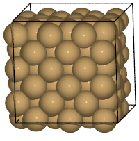
結果を可視化してみると以下のようになります。
ここではread関数に index="::100" を指定することでTrajectoryファイルから間隔を間引いた結果に対して可視化しています。 Cuは固体の構造を保っており、大きく動いているわけではありませんが、振動の動きによりセルサイズに変化があることがわかります。
[2]:
from ase.io import Trajectory, read
from pfcc_extras.visualize.povray import traj_to_apng
from IPython.display import Image


traj = read("./output/ch6/fcc-Cu_3x3x3_NPT_EMT_0900K.traj", index="::100")
traj_to_apng(traj, f"output/ch6/Fig6-3_fcc-Cu_3x3x3_NPT_EMT_0900K.png", rotation="10x,-10y,0z", clean=True, n_jobs=16)

Image(url="output/ch6/Fig6-3_fcc-Cu_3x3x3_NPT_EMT_0900K.png")
[Parallel(n_jobs=16)]: Using backend ThreadingBackend with 16 concurrent workers.
[Parallel(n_jobs=16)]: Done  12 out of  21 | elapsed:    5.8s remaining:    4.4s
[Parallel(n_jobs=16)]: Done  21 out of  21 | elapsed:    7.2s finished
[2]:
[3]:
from ase.io import Trajectory, read
from pfcc_extras.visualize.view import view_ngl


traj = read("./output/ch6/fcc-Cu_3x3x3_NPT_EMT_0900K.traj", index="::100")
view_ngl(traj, replace_structure=True)
[3]:
熱浴の時定数\(\tau_t\)は20 fs、圧力制御パラメーターであるpfactorは2e6 GPa\(\cdot\)fs\(^2\)としています。上記の計算条件で熱平衡状態にするため300 Kで20 psのNPT-MDシミュレーションを行った際のセル体積の時間変化の様子を確認してみましょう。以下のようなコードで特定温度におけるMDシミュレーションの結果であるtrajファイルを解析出来ます。
[4]:
import matplotlib.pyplot as plt
from pathlib import Path
from ase.io import read,Trajectory

time_step = 0.01  # Time step size in ps between each snapshots recorded in traj
traj = Trajectory("./output/ch6/fcc-Cu_3x3x3_NPT_EMT_0300K.traj")

time = [ i*time_step for i in range(len(traj)) ]
volume = [ atoms.get_volume() for atoms in traj ]

# Create graph
fig = plt.figure(figsize=(8,3))
ax = fig.add_subplot(1, 1, 1)
ax.set_xlabel('time (ps)')  # x axis label
ax.set_ylabel('Cell volume (Å^3)')  # y axis label
ax.plot(time,volume, alpha=0.5)
ax.set_ylim([1100,1400])
#plt.savefig("filename.png")  # Set filename to be saved
plt.show()
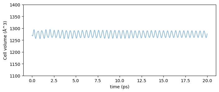
上記コードを実行すると、以下のような解析結果が得られます。
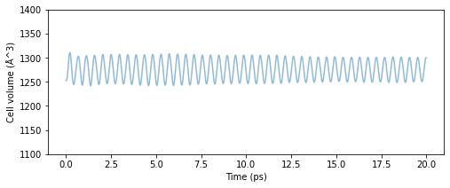
Fig.6-3a. Time evolution of cell volume. (fcc-Cu_3x3x3, @300 K and 1 bar)
NPTアンサンブルで計算することでセル体積が約4%程の範囲で振動することが見て取れます。今回の計算対象は立方晶であるため、この体積の幾何平均から結晶の格子定数を計算出来ます。200 Kから1000 Kまで実行し、その各温度での規格化した格子定数の平均値をプロットすると以下の結果が得られます。(平衡状態に達したあとの格子定数を計算したいため、np.mean(vol[int(len(vol)/2):])**(1/3) の部分では、Trajectoryの後半半分のみを使用して、体積から格子定数を計算しています。)
[5]:
import matplotlib.pyplot as plt
import numpy as np
from pathlib import Path
from ase.io import read,Trajectory

time_step = 10.0  # Time step size between each snapshots recorded in traj
paths = Path("./output/ch6/").glob(f"**/fcc-Cu_3x3x3_NPT_{calc_type}_*K.traj")
path_list = sorted([ p for p in paths ])

# Temperature list extracted from the filename
temperature = [ float(p.stem.split("_")[-1].replace("K","")) for p in path_list ]
print("temperature = ",temperature)

# Compute lattice parameter
lat_a = []
for path in path_list:
    print(f"path = {path}")
    traj = Trajectory(path)
    vol = [ atoms.get_volume() for atoms in traj ]
    lat_a.append(np.mean(vol[int(len(vol)/2):])**(1/3))

print("lat_a = ",lat_a)

# Normalize relative to the value at 300 K
norm_lat_a = lat_a/lat_a[1]
print("norm_lat_a = ",norm_lat_a)

# Plot
fig = plt.figure(figsize=(4,4))
ax = fig.add_subplot(1, 1, 1)
ax.set_xlabel('Temperature (K)')  # x axis label
ax.set_ylabel('Normalized lattice parameter')  # y axis label
ax.scatter(temperature[:len(norm_lat_a)],norm_lat_a, alpha=0.5,label=calc_type.lower())
ax.legend(loc="upper left")
temperature =  [200.0, 300.0, 400.0, 500.0, 600.0, 700.0, 800.0, 900.0, 1000.0]
path = output/ch6/fcc-Cu_3x3x3_NPT_EMT_0200K.traj
path = output/ch6/fcc-Cu_3x3x3_NPT_EMT_0300K.traj
path = output/ch6/fcc-Cu_3x3x3_NPT_EMT_0400K.traj
path = output/ch6/fcc-Cu_3x3x3_NPT_EMT_0500K.traj
path = output/ch6/fcc-Cu_3x3x3_NPT_EMT_0600K.traj
path = output/ch6/fcc-Cu_3x3x3_NPT_EMT_0700K.traj
path = output/ch6/fcc-Cu_3x3x3_NPT_EMT_0800K.traj
path = output/ch6/fcc-Cu_3x3x3_NPT_EMT_0900K.traj
path = output/ch6/fcc-Cu_3x3x3_NPT_EMT_1000K.traj
lat_a =  [10.821187657763522, 10.84284171781325, 10.866195382765163, 10.88834101681545, 10.91184951417741, 10.937661285868403, 10.958914931081702, 10.988423059467703, 11.016341565694251]
norm_lat_a =  [0.99800292 1.         1.00215383 1.00419625 1.00636436 1.0087449
 1.01070505 1.01342649 1.01600133]
[5]:
<matplotlib.legend.Legend at 0x7f2643b7a210>
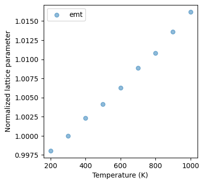
上記のコードを実行すると以下のようなプロットが得られます。
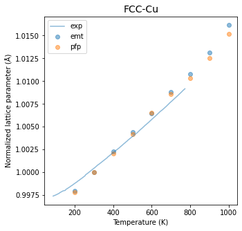
Fig.6-3b. Normalized lattice parameter as a function of temperature.
Experimental data is taken from Reference [4].
この結果にはさらにPFPを用いた計算結果、および参考までに実験値を比較対象としています。EMTおよびPFPのデータ共に非常に良い一致を示しており、小さな差ではありますがPFPはより実験値に近い傾向を示しています。
この規格化した格子定数の温度依存性から線熱膨張係数(CTE、\(\alpha\))を以下の関係式をもちいて算出します。
ここで\(\alpha\)が線熱膨張係数で、\(a(T)\)と\(a_{RT}\)は温度\(T\)と室温における格子定数です。以下がASAP3-EMT、PFP、実験値[4]のサマリーです。
\(\alpha\) ( \(10^{-5}\) /K) |
|
|---|---|
emt |
2.23 |
pfp |
2.13 |
exp |
1.74 |
計算誤差を考えると、いずれの計算結果も実験値とリーズナブルな範囲で一致していると考えてよいと思います。
このような手法でNPTアンサンブルのMDシミュレーションを用いることによって熱膨張係数を算出することが可能です。
最後に補足として言及しますと、「液体や気体の熱膨張も同様の手法で再現できるのでは?」と考えるかと思います。原理的には確かにその通りなのですが、現時点では再現性の良いモデルというのは限定的と思われます。古典力場で特定の液体や気体のみに特化したモデルは存在するのかもしれませんが、第一原理計算を用いた場合、液体や気体では固体に比べて非常に小さい分子間相互作用の精度が重要になり、現在ではそのような精度の量子化学計算自体が非常に困難です。特にNNPを作成する際には膨大な計算データが必要になり、高精度な量子化学計算を多量に行うのは現時点であまり現実的ではありません。従って今後この領域での精度が高いモデルの開発が期待されるところです。
[Advanced] Parrinello-Rahman barostatのパラメーター依存性
NPTアンサンブルでのMDシミュレーションを行う際にpfactorというパラメーターを設定する必要があり、適切な値の範囲が 10\(^6\) GPa\(\cdot\)fs\(^2\)から10\(^7\) GPa\(\cdot\)fs\(^2\)付近という説明がありました。ご参考までにpfactorの値を変化し際の結果を以下に示します。計算対象は上記と同じfcc-Cuの3x3x3 unit cellsで、温度は300 Kです。
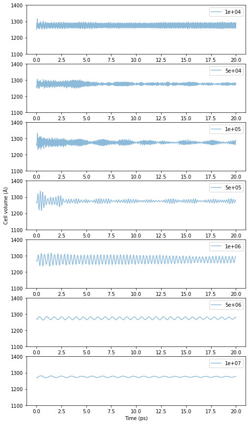
Fig.6-3c. Time evolution of cell volume as a function of pfactor.
pfactorが小さい領域では高速でセル体積が振動しており、高周波と低周波の振動が混在していて挙動が不安定な領域もあるのであまり好ましくありません。pfactorが大きくなるにつれて振動の周期が徐々に長くなり、小さなpfactorの計算初期で起きるの大きなセル体積の変化も殆ど見られません。明確にpfactorのどの値から使うと良いという指標があるわけではないですが、10\(^6\) Ga\(\cdot\)fsec\(^2\)以上であれば小さな振動は確認できるものの中央値は相変わらず安定しているようです。上限についても同様で明確な基準はなく、pfactorが大きいと振動周期が長くなり扱いづらいので、上記の例に関していえば10\(^6\)から10\(^7\)ぐらいが妥当な領域かと考えます。
[Advanced] Berendsen barostatのパラメーター依存性
Berendsen barostatを用いた計算方法について説明します。Berendsen barostatは以下の方程式に従って圧力の時間発展が計算されます。(導出の詳細は参考文献[5]をご覧ください。)
上式から明らかなように、Berendsen圧力制御法では指数関数的に系の各瞬間における圧力を外圧\(\mathbf{P}_o\)に近づけていきます。その速度は時定数\(\tau_P\)により制御されます。
各MDステップ毎に、各原子の座標とセルベクトルは以下の式で表される係数でスケーリングされます。
熱浴のコントロールの際に\(\tau_T\)が時定数だったように、圧力制御法でも適切な時定数\({\tau_P}\)を設定してやる必要があります。それでは実際の計算事例を見てみましょう。
ASEの機能であるNPTBerendsenクラスを用いるとdynamicsを定義するオブジェクトは以下の形で記述されます。
[6]:
from ase.md.nptberendsen import NPTBerendsen

dyn = NPTBerendsen(
    atoms,
    time_step*units.fs,
    temperature_K = temperature,
    pressure_au = 1.0 * units.bar,
    taut = 5.0 * units.fs,
    taup = 500.0 * units.fs,
    compressibility_au = 5e-7 / units.bar,
    logfile = log_filename,
    trajectory = traj_filename,
    loginterval=num_interval
)
圧力の異方性を考慮できるInhomogeneous_NPTBerendsenもほぼ同様の設定です。(クラス名をNPTBerendsenからInhomogeneous_NPTBerendsenとすることで利用可能です。)1点異なるのはmaskが設定でき、mask=(1, 1, 1)とするとa,b,c方向全て独立して変化可能です。このtupleの要素を0と設定することでその方向でcellが固定されます。
いずれのBerendsen barostatでも注意が必要なのは温度、圧力のような計算条件以外に、圧力制御時定数(taup、\(\tau_P\))や圧縮率(compressibility、\(\beta_T\))と呼ばれるパラメーターを設定する必要があることです。それぞれの値に対するセル体積の時間変化の依存性を300 Kにおけるfcc-Cuの例を用いて確認します。まずは\(\tau_P\)の方からみてみます。
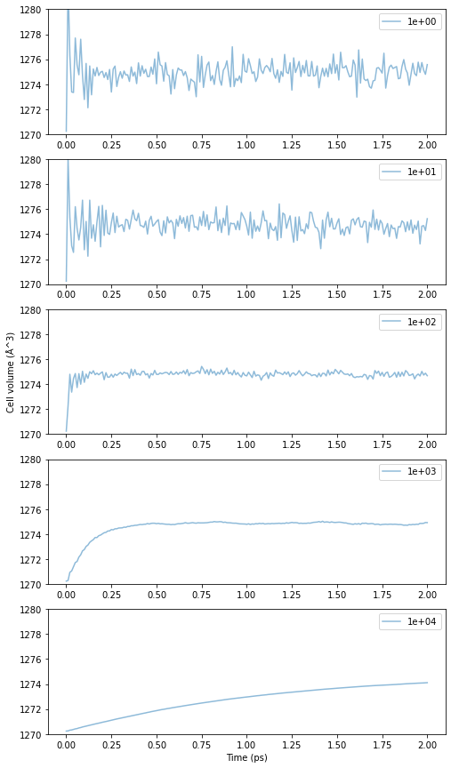
Fig.6-3d. Time evolution of cell volume as a function of \(\tau_P\).
時定数が小さいほど振動の周期が不安定で大きく暴れ、逆にあまり大きくとりすぎると変化があまりに緩やかで平衡に至るまでの時間がかかります。この辺りは熱浴法の時定数と同じ考え方です。力学的にfcc-Cuと類似の系に関しては体積変化の安定性と収束性から\(\tau_P\)は10\(^2\) fsから10\(^3\) fs付近が適切なようです。
次に\(\beta_T\)に対する依存性です。結果は以下のとおりです。
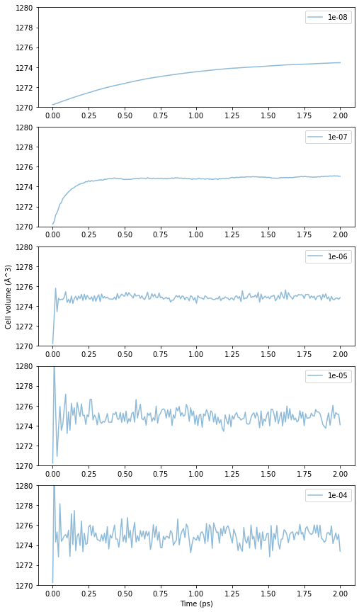
Fig.6-3e. Time evolution of cell volume as a function of \(\beta_T\).
\(\beta_T\)が小さいほど収束が非常に遅く、高い値にあるほど不安定になっていく様子がうかがえます。グラフの傾向から\(\beta_T\)は10\(^{-7}\)から10\(^{-6}\)fs位が良さそうです。
\(\tau_P\)と\(\beta_T\)に関してはいずれも厳密に正しい値というものは無く、おおよそ桁で値を変えた時にこの程度傾向が変化するということを理解しておけば概ね問題はなさそうです。
最後に補足すると、これらの数値はあくまでfcc-Cuのような金属で密な構造を持つ物質について適用出来ますが、もし全く異なる系統の物質(例えばポリマー、液体、気体等)をNPTで扱いたいとなれば事前検討でこれらの適切な値の領域を確認しておく必要があります。手間を惜しんで事前検討を省くと意図しない結果が得られて余計に時間がかかるなどになりかねないので、通常、新しい材料系に取り組む際は注意されることをお勧めします。
参考文献
[1] M.E. Tuckerman, “Statistical mechanics: Theory and molecular simulation”, Oxford University Press (2010) ISBN 978-0-19-852526-4. https://global.oup.com/academic/product/statistical-mechanics-9780198525264?q=Statistical%20mechanics:%20Theory%20and%20molecular%20simulation&cc=gb&lang=en#
[2] Melchionna S. (2000) “Constrained systems and statistical distribution”, Physical Review E 61 (6) 6165 https://journals.aps.org/pre/abstract/10.1103/PhysRevE.61.6165
[3] S. Melchionna, G. Ciccotti, B.L. Holian, “Hoover NPT dynamics for systems varying in shape and size”, Molecular Physics, (1993) 78 (3) 533 https://doi.org/10.1080/00268979300100371
[4] F.C. Nix, D. MacNair, “NIST:The Thermal Expansion of Pure Metals: Copper, Gold, Aluminum, Nickel, and Iron” https://materialsdata.nist.gov/handle/11256/32
[5] H. J. C. Berendsen, J. P. M. Postma, W. F. van Gunsteren, A. DiNola, and J. R. Haak, “Molecular dynamics with coupling to an external bath”, J. Chem. Phys. (1984) 81 3684 https://aip.scitation.org/doi/10.1063/1.448118